Sage Journals: Discover world-class research

Abstract

Imperfection in a bonding point can affect the quality of an entire integrated circuit. Therefore, a time–frequency analysis method was proposed to detect and identify fault bonds. First, the bonding voltage and current signals were acquired from the ultrasonic generator. Second, with Wigner–Ville distribution and empirical mode decomposition methods, the features of bonding electrical signals were extracted. Then, the principal component analysis method was further used for feature selection. Finally, an artificial neural network was built to recognize and detect the quality of ultrasonic wire bonding. The results showed that the average recognition accuracy of Wigner–Ville distribution and empirical mode decomposition was 78% and 93%, respectively. The recognition accuracy of empirical mode decomposition is obviously higher than that of the Wigner–Ville distribution method. In general, using the time–frequency analysis method to classify and identify the fault bonds improved the quality of the wire-bonding products.

Keywords

Ultrasonic wire bonding quality detection time–frequency analysis feature extraction feature selection pattern recognition

Introduction

With the development of integrated circuits, advanced packaging technology has been constantly promoted to meet the requirements and challenges of various new semiconductor processes and materials.^1,2 The internal lead interconnection technology in microelectronic packaging is the key technology to realize the interconnection between the internal chip and the external pin and between the chips.^3,4 It plays an important role in establishing the electrical connection between the chip and the external and ensuring the smooth input and output between the chip and the outside. It is also the key to the whole backchannel packaging process. Both the facts of the packaging industry for many years and the predictions of the authorities indicate that ultrasonic lead bonding will continue for the foreseeable future. It will be the main way of lead interconnection in microelectronic packaging. The ultrasonic lead bonding method is to bond the two ends of the fine metal lead on the chip and the substrate bonding pad respectively to form its electrical connection. The ultrasonic lead bonding technology is dominant in the interconnection of microelectronic packaging due to its simple process, low cost, and suitable for various packaging forms, which realize the interconnection of the above packages. In addition, with the development of high-speed and high-precision wire bonding, higher requirements are placed on the reliability of the bonding process and the quality of the bonding. Bonding point imperfections can affect the quality of the entire integrated circuit.^5,6 Therefore, detecting the bonding quality is of great significance.⁷

Over the years, scholars have conducted extensive research on quality detection of ultrasonic bonding.⁸ The techniques are mainly based on the detection of bonding process information related with bond quality. Southern Methodist University,⁹ Seoul National University,¹⁰ and the Xi’an Jiaotong University¹¹ have used image processing and recognition methods to detect the quality of bonding points. Compared with manual visual inspection, these methods have the characteristics of high speed and high precision. The main disadvantage of the above detection method is that this technology is offline and the state of the bonding point and the defects of the process parameters cannot be reported in real time, which is not conducive to the timely adjustment of the process. For on-line quality detection technologies, Long et al.¹² used the noncontact measurement method of a Doppler vibrometer to extract the vibration signal at the end of a cleaver during bonding and identified whether the bonding process was successful in time–frequency domain analysis. Zhong and Goh¹³ studied the feature extraction method of bonding tool vibration signals and applied it to the bonding quality detection process. Zhong and Goh¹³ have also conducted extensive research on the vibration testing of bonding tools and the evaluation of bonding quality. Gobel et al. used sensors to determine the changes in the position of a bonding tool during the bonding process and determined that the metal lead was not in conformity with the deformation range in poor quality bonding. Mayer and Schwizer¹⁴ used a sensor to detect the temperature and force in the X, Y, and Z axes around a pad and evaluated the bonding quality according to the change in the temperature signal. The above on-line detection techniques reveal the intimate relationship between bond quality and factors such as bonding interface friction, capillary vibration, and horn vibration. Some signal processing methods are used for extracting features and identifying bond quality. However, the rigorous demands for special sensor designing and installing increase the difficulty of applying the techniques to a factory settings.^15–17

The new method based on the time–frequency analysis was proposed to detect and identify fault bonds in this article. It not only enables real-time feedback and adjustment but also does not require an additional sensor, and uses the inherent self-sensor characteristics of the piezoelectric transducer system to detect the wire-bonding signal. We extend the technique of detecting the bonding process via analysis of voltage and current from the ultrasonic generator supply. In order to characterize the transient property and extract the local, tiny changes in the electrical signals, a new technology, including time–frequency analysis method, feature extraction method and pattern recognition method, was studied and used. First, the bonding voltage and current signals were acquired from the ultrasonic generator. Second, with Wigner–Ville distribution (WVD) and empirical mode decomposition (EMD) methods, the features of bonding electrical signals were extracted. Third, principal component analysis (PCA) is carried out to remove the redundant information and leave the component representing the main information of the bonding process. Finally, an artificial neural network was built to recognize and classify the four types of bonding failure modes. In general, by using joint time–frequency distribution and EMD to decompose and extract ultrasonic electrical signals, the extracted features were used to classify and identify the four types of failure modes, which improved the quality of the wire-bonding products.

Time–frequency analysis methods

Time–frequency analysis is an abbreviation of real-time frequency joint domain analysis and is used as a powerful tool for analyzing time-varying nonstationary signals.¹⁸ The time–frequency analysis method provides joint distribution information of the time domain and the frequency domain, clearly describes the relationship of the signal frequency with time, and offers an obvious advantage in the study of transient nonstationary characteristic signals. Especially in the field of feature extraction, time–frequency analysis methods can intuitively analyze ultrasonic electrical signals. Commonly used time–frequency representations can be categorized as linear or nonlinear. Typical linear time–frequency representations include short-time Fourier transforms and continuous wavelet transforms. Typical nonlinear time–frequency representations include the WVD and Cohen distribution. This article will use time–frequency analysis to decompose and extract the signal, including WVD and EMD.

WVD

Assume that signals x(t) and y(t) are continuously changing time signals and that X(ω) and Y(ω) represent respective Fourier transforms, the joint WVD distribution of x(t) and y(t) can be defined as

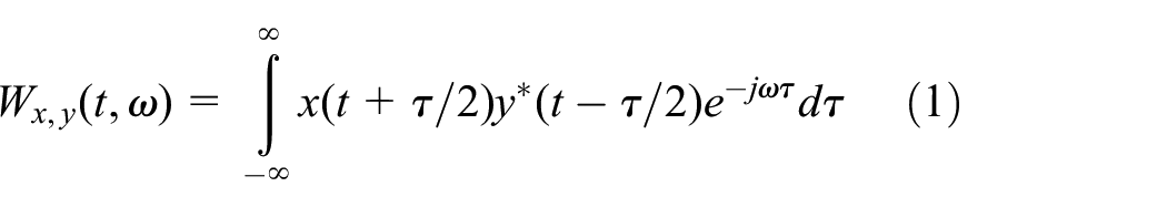
W_{x, y} (t, ω) = \int_{- \infty}^{\infty} x (t + τ / 2) y^{*} (t - τ / 2) e^{- j ω τ} d τ

(1)

The self-WVD time–frequency distribution of the signal can be defined as

W_{x} (t, ω) = \int_{- \infty}^{\infty} x (t + τ / 2) x^{*} (t - τ / 2) e^{- j ω τ} d τ

(2)

Similarly, using the frequency domain functions X(ω) and Y(ω), the joint WVD distribution of the time domain variables x(t) and y(t) can be obtained

W_{X, Y} (ω, t) = \frac{1}{2 π} \int_{- \infty}^{\infty} X (ω + ζ / 2) Y^{*} (ω - ζ / 2) e^{- jt ζ} d ζ

(3)

W_{X} (ω, t) = \frac{1}{2 π} \int_{- \infty}^{\infty} X (ω + ζ / 2) X^{*} (ω - ζ / 2) e^{- jt ζ} d ζ

(4)

W_{x} (t, ω) = W_{X} (ω, t)

(5)

W_{x, y} (t, ω) = W_{X, Y} (ω, t)

(6)

Equation 3 can be regarded as the Fourier transform of the signal x(t) and y(t) cross-correlation function $r_{x, y} (t, τ) = x (t + τ / 2) y^{*} (t - τ / 2)$ to $τ$ ; Equation 4 can be regarded as the Fourier transform of the signal x(t) autocorrelation function $r_{x} (t, τ) = x (t + τ / 2) x^{*} (t - τ / 2)$ to $τ$ .

EMD

The specific process of EMD of any real signal x(t) is as follows: first determine all the extreme points on x(t), then connect all the maximum points and all the minimum points with a curve, and remember that the two curves obtained by fitting the extreme signal points are the combination of upper x(t) envelope $f_{\max} (t)$ and lower envelope $f_{\min} (t)$ . Let the average value of $f_{\max} (t)$ and $f_{\min} (t)$ be denoted as m(t), and the difference between x(t) and m(t), be denoted as h(t)

x (t) - m (t) = h (t)

(7)

Ideally, $h (t)$ should be an IMF because the construction process of h(t) must satisfy the two conditions of the intrinsic mode functions (IMF). However, due to the complexity of the actual signal, in general, h(t) is not a stable data series. Therefore, consider h(t) as a new $x (t)$ and repeat the above operation until h(t) meets a certain inherent pattern

c_{1} (t) = h (t)

(8)

s (t) - c_{1} (t) = r (t)

(9)

Treat $r (t)$ as a new $x (t)$ and repeat the above process to obtain the second IMF, the third IMF, and so on. When $c_{n}$ or $r (t)$ meets the given sieving end condition, obtaining the decomposition formula

s (t) = \sum_{i = 1}^{n} c_{i} (t) + r_{n} (t)

(10)

where $r (t)$ is the residual function and represents the average trend of the signal.

Bonding quality detection

During the bonding process, the fault bonding mainly includes the following four types as shown in Figure 1: (1) position-off bonding, which is mainly manifested in the improper positioning between the bonding point and the substrate, and the formed bonding point is not completely stuck in the middle of the substrate, and will occur short circuit. (2) Wire breakage failure, when there is no metal ball at the tip of the bonding tool, resulting in direct contact friction between the bonding tool and the substrate. (3) Noncontact bonding, the main reason is that the chip layer of the substrate falls off or the positioning of the bonding system is inaccurate, which causes no contact friction between the bonding tool and the metal ball and the substrate. (4) The root peeling bonding point, after the bonding is completed, the formed bonding point falls off directly or the shear force is insufficient to fall off.

Figure 1.

Four bonding failure modes: (a) position-off bonding, (b) wire breakage, (c) noncontact bonding, and (d) root peeling bonding.

A schematic diagram of the entire process is shown in Figure 2. First, the ultrasonic generator coupling signal is obtained during the bonding process and then the characteristics of the bonding state information are extracted according to the need to detect the corresponding bonding quality.¹⁹ Finally, pattern recognition technology is used to identify the bonding quality.

Figure 2.

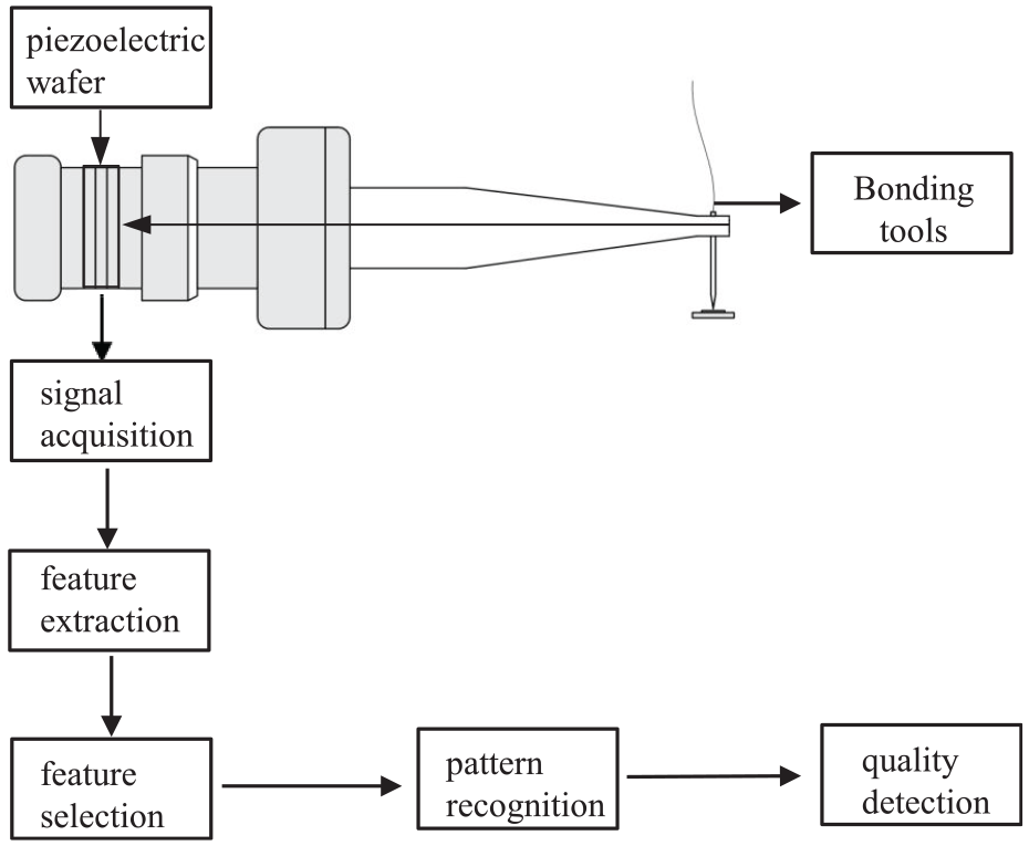
Schematic diagram of quality detection process.

Signal acquisition

When the bonding is about to start, there is a positive transition signal caused by the impact between the bonding tool and the substrate in the ultrasonic voltage signal during the bonding process. The transition signal is basically maintained between 0.03 and 0.05 V. However, during the pre-bonding stage, except for this transition signal, the voltage signal fluctuates between −0.001 and 0.001 V, and these signals can be regarded as noise signals. Figure 3 shows the waveform of the voltage signal during the bonding process. It can be observed in the figure that at a certain time point before the bonding, there are obvious transition signals, which provide opportunities for triggering acquisition. Using the transition signal as a trigger signal, the voltage and current signals can be collected during the bonding process, which ensures the simultaneous collection of voltage and current as well as the capturing of signals. A set of ultrasonic voltage and current signals collected during the bonding process is shown in Figure 4.

Figure 3.

Trigger principle of ultrasonic electric signal.

Figure 4.

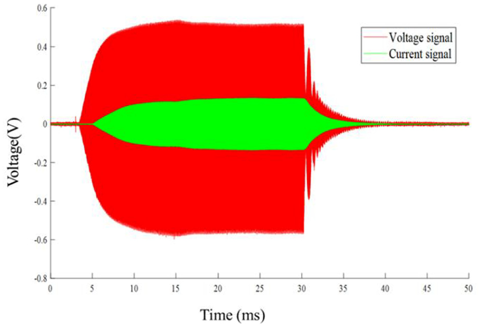
Ultrasonic voltage and current signal.

To achieve consistency of different bonding signals over time, one starts with the transition signal, then intercepts the signals uniformly, and finally extracts the feature. Figure 5 shows the waveform and spectrum characteristics of a group of typical ultrasonic electrical signals. It can be seen that its transient characteristics are obvious. In addition, it can be seen from the spectrum diagram of voltage and current signals that the energy of ultrasonic electrical signals is mainly concentrated in the first third octave (65 kHz).

Figure 5.

Ultrasonic voltage and current signals and spectrum.

Feature extraction

To extract features from the time–frequency distribution of the signal, this article uses the time–frequency distribution contour area method to extract the features of the ultrasonic electrical signal²⁰ and the adaptive mode decomposition of the ultrasonic electrical signal using EMD.

Feature extraction of ultrasonic electrical signal based on WVD

Based on WVD, the joint time–frequency distribution of voltage and current signals in four failure modes is obtained as showed in Figure 6. It can be seen from the time–frequency distribution diagrams that the four types of bonding failure modes are not visually obvious, the voltage amplitude of the position-off bonding and noncontact bonding is small (0.4 V), and the current amplitude is relatively large (0.15 A). The voltage amplitude of the bonding point for wire breakage failure and root peeling is approximately 0.5 V, and the current amplitude is approximately 0.12 A. The ultrasonic signal amplitude at the root of peeling bonding point is relatively severe.

Figure 6.

WVD distribution of ultrasonic electrical signals in four failure modes: (a) position-off bonding, (b) wire breakage, (c) noncontact bonding, (d) root peeling bonding, (e) position-off bonding, (f) wire breakage, (g) noncontact bonding, and (h) root peeling bonding.

To further extract features from the time–frequency distribution, the time–frequency distribution of the four types of failure signals appears as an intercepted contour line, and the number of equal divisions is 18, as showed in Figure 7. As the frequency doubling component of the ultrasonic current signal is very small, only the contour line (60–66 kHz, where the ultrasonic loading frequency is 63.5 kHz) at the fundamental frequency is given in the contour plot. It can be seen from the figure that the contours of the four types of bond failure modes are very similar and difficult to distinguish.

Figure 7.

Time–frequency distribution contours of four failure modes: (a) position-off bonding, (b) wire breakage, (c) noncontact bonding, (d) root peeling bonding, (e) position-off bonding, (f) wire breakage, (g) noncontact bonding, and (h) root peeling bonding.

In order to extract the feature from the time–frequency distribution of the signal, this article uses the time–frequency distribution contour area method to extract the feature from the time–frequency distribution of the ultrasonic electrical signal. A total of 36 feature values were extracted from the time–frequency distribution of a group of ultrasonic signals due to the simultaneous feature extraction of ultrasonic voltage and current signals. The results are shown in Table 1.

Table 1.

Extraction results of WVD.

ModeFeature	Position-off bonding		Wire breakage		Noncontact bonding		Root peeling bonding
	U (V)	I (A)	U (V)	I (A)	U (V)	I (A)	U (V)	I (A)
$W_{1 S}$	106.45	74.66	107.32	74.37	110.75	75.37	103.05	72.36
$W_{2 S}$	105.12	72.19	105.66	72.55	108.19	74.18	102.1	70.25
$W_{3 S}$	103.26	70.96	104.29	70.83	106.26	72.46	100.57	68.67
$W_{4 S}$	99.87	67.16	100.69	68.52	103.87	68.58	97.37	66.89
$W_{5 S}$	94.76	65.32	95.76	65.64	97.56	67.97	93.76	63.26
$W_{6 S}$	93.12	63.19	93.87	63.58	95.39	64.55	91.12	61.01
$W_{7 S}$	91.77	62.87	92.17	62.74	94.22	63.56	90.82	60.77
$W_{8 S}$	88.99	61.96	89.75	60.87	92.69	62.24	89.68	58.91
$W_{9 S}$	87.36	58.74	87.66	58.56	89.36	59.28	88.67	56.78
$W_{10 S}$	86.69	56.21	85.37	56.38	87.44	58.34	87.57	54.41
$W_{11 S}$	83.62	52.98	83.19	53.27	85.62	54.54	81.86	52.65
$W_{12 S}$	81.07	46.12	81.56	44.19	83.19	49.12	79.03	44.19
$W_{13 S}$	74.19	35.18	70.66	34.18	78.39	38.18	73.2	32.17
$W_{14 S}$	58.66	32.68	62.48	31.58	66.58	33.79	55.89	32.63
$W_{15 S}$	51.09	24.17	55.49	26.19	58.49	27.27	50.54	21.15
$W_{16 S}$	42.17	21.67	43.19	22.65	47.13	23.69	40.78	19.6
$W_{17 S}$	31.74	16.54	36.84	13.59	36.89	19.58	23.55	16.94
$W_{18 S}$	11.26	9.77	16.29	10.69	21.58	15.1	5.23	13.7

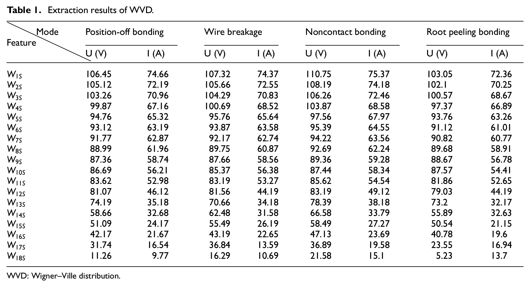
WVD: Wigner–Ville distribution.

The specific implementation process is as follows: W is set as the time–frequency distribution of ultrasonic electrical signal, and W is intersected on the x–y plane based on the amplitude and height of W. Here, n interception is assumed to be selected. After the interception, n groups of contour planes (including those with amplitude of 0) can be obtained. By taking the area contained in each contour line as the eigenvalue, the following eigenvectors can be obtained

F_{W} = [W_{1 s}, W_{2 s}, \dots, W_{ns}]

(11)

where $F_{W}$ represents the feature vector of time–frequency distribution, $W_{1 s}$ , $W_{2 s}$ , and $W_{ns}$ represent the area contained in the contour line.

Feature extraction of ultrasonic electrical signal based on EMD

Based on EMD,²¹ decomposed results of ultrasonic voltage and current signals are obtained at 6 IMF components as showed in Figure 8. The “res.” represents the EMD residual signal (the scale is enlarged by 10 times), and the horizontal coordinate represents time (t/ms). It can be seen from the figure that the difference of the components of each mode is not very obvious.

Figure 8.

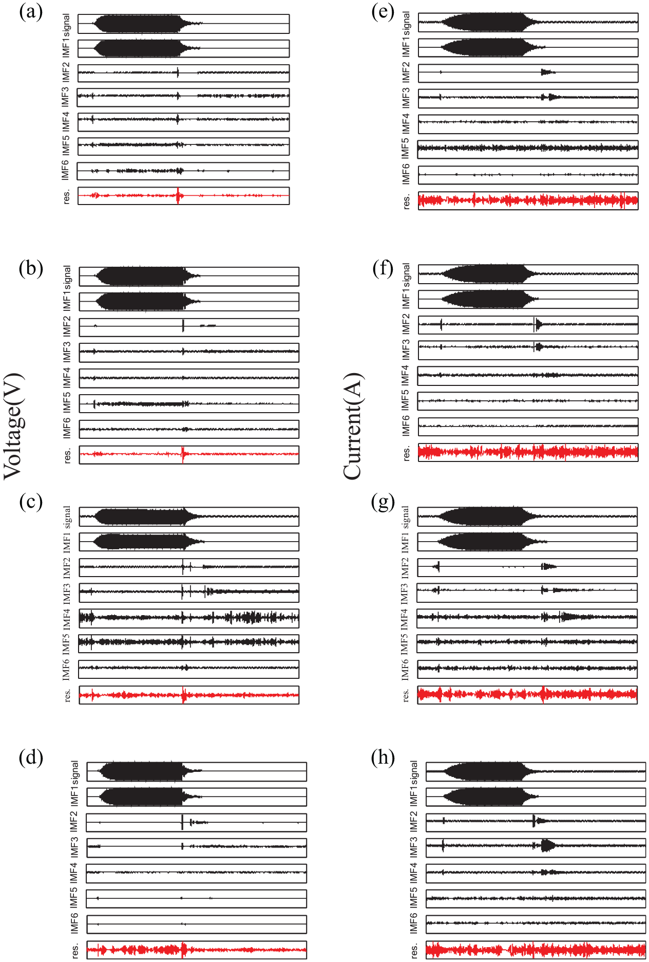
EMD results of four bond failure signals: (a) position-off bonding, (b) wire breakage, (c) noncontact bonding, (d) root peeling bonding, (e) position-off bonding, (f) wire breakage, (g) noncontact bonding, and (h) root peeling bonding.

In this article, the IMF component is obtained using the EMD method, then performs feature extraction on these IMF components: 500 sets of experimental data (125 sets of data for each model) were calculated to obtain the average results (Table 2).

Table 2.

EMD feature extraction results.

ModeFeature	Position-off bonding		Wire breakage		Noncontact bonding		Root peeling bonding
	U (V)	I (A)	U (V)	I (A)	U (V)	I (A)	U (V)	I (A)
$E_{IMF 1}$	0.2854	0.1679	0.3699	0.2178	0.2256	0.1259	0.4498	0.1129
$E_{IMF 2}$	0.0638	0.0495	0.1135	0.0793	0.0339	0.0195	0.1962	0.0795
$E_{IMF 3}$	0.0148	0.0096	0.0798	0.0376	0.0177	0.0376	0.0979	0.0568
$E_{IMF 4}$	0.0195	0.0069	0.0585	0.026	0.0045	0.0259	0.0578	0.0667
$E_{IMF 5}$	0.0087	0.0098	0.0327	0.0188	0.0017	0.0078	0.0483	0.0067
$E_{IMF 6}$	0.0062	0.0067	0.0099	0.0003	0.0002	0.0009	0.0047	0.0013
$S_{IMF 1}$	63.254	63.254	62.798	62.798	63.954	63.954	62.964	62.964
$S_{IMF 2}$	22.486	22.486	36.473	36.473	11.975	11.975	47.489	47.489
$S_{IMF 3}$	16.535	16.535	29.692	29.692	7.935	7.935	25.537	25.537
$S_{IMF 4}$	6.987	6.987	18.469	18.469	1.587	1.587	11.387	11.387
$S_{IMF 5}$	0.965	0.965	7.168	7.168	0.337	0.337	0.907	0.907
$S_{IMF 6}$	0.298	0.298	0.179	0.179	0.101	0.101	0.833	0.833

EMD: empirical mode decomposition.

The specific implementation process is as follows: Let $IM F_{i} = [IM F_{1}, IM F_{2}, \dots, IM F_{n}]$ be the IMF component obtained by EMD method. Its eigenvectors are defined as follows

\begin{matrix} F_{E} = [E_{IMF 1}, E_{MMF 2}, \dots, E_{IMFn}, S_{MNF 1}, S_{IMF 2}, \dots, S_{IMFn}], \\ n = 1, 2, 3, \dots \end{matrix}

(12)

$F_{E}$ represents the feature vector, $E_{IMF 1}$ , $E_{MMF 2}$ , and $E_{IMFn}$ represent the energy characteristics of each model component, $S_{MNF 1}$ , $S_{IMF 2}$ , and $S_{IMFn}$ represent the frequency characteristics of each mode component, and n represents number of mode components.

Feature selection

In order to eliminate the correlation between extracted features and achieve feature dimensionality reduction, feature selection is required after feature extraction. Therefore, PCA of the original feature data is carried out in this article to remove the redundant information and leave the component representing the main information of the bonding process, which can reduce the computational complexity of pattern recognition and increase the recognition precision.

The specific calculation process of PCA is as follows: Let $X = [x_{1}, x_{2}, \dots, x_{n}]^{T}$ be the original feature matrix; $Y = [y_{1}, y_{2}, \dots, y_{n}]$ is the normalized feature matrix, where $y_{i}$ is given by

y_{i} = \frac{x_{i} - \bar{x_{i}}}{\sqrt{σ_{i}}}

(13)

$\bar{x_{i}} = (1 / m) \sum_{j = 1}^{m} x_{ij}$ , $σ_{i} = 1 / (m - 1) \sum_{j = 1}^{m} {(x_{ij} - \bar{x_{i}})}^{2}$ , and m are the dimensions of original feature variables.

R_{y} = {\begin{matrix} 1 & r_{12} & \dots & r_{1 n} \\ r_{21} & 1 & \dots & r_{2 n} \\ ⋮ & ⋮ & ⋱ & ⋮ \\ r_{n 1} & r_{n 2} & \dots & 1 \end{matrix}}

(14)

where $r_{ij} = E [y_{i} y_{j}] (i, j = 1, 2, \dots, n)$ denotes cross-correlation and E[ ] denotes the mathematical expectation.

If $| R_{y} - λ I | = 0$ , I is the identity matrix, and $λ$ is the eigenvalues of $R_{y}$ .

Find n non-negative real roots and arrange them in descending order

λ_{1} \geq λ_{2} \geq \dots \geq λ_{n} \geq 0

(15)

Bring $λ_{i} (i = 1, 2, \dots, n)$ into the following equation to obtain the eigenvector $u_{i} (i = 1, 2, \dots, n)$

(R_{y} - λ_{i} I) u_{i} = 0

(16)

Bring $u_{i} (i = 1, 2, \dots, n)$ into the following equation to obtain the principal component

z_{i} = u_{i}^{T} y_{i}

(17)

The contribution rate of the ith principal component is defined as follows

P_{λ} = \frac{λ_{i}}{\sum_{i = 1}^{n} λ_{i}}

(18)

The cumulative contribution rate of the first k principal components is defined as follows

S_{λ} = \frac{\sum_{i = 1}^{k} λ_{i}}{\sum_{i = 1}^{n} λ_{i}}

(19)

In this way, after the above calculation process, a set of uncorrelated feature variables $z_{i} (i = 1, 2, \dots, n)$ will be obtained. By calculating the cumulative contribution rate, the first k principal components are selected and $z_{i} (i = 1, 2, \dots, k; k \leq n)$ represents the original feature variable used to achieve dimensionality reduction and correlation elimination.

Generally, the first k principal components when the cumulative contribution rate is greater than 95% represent the original feature vector. Perform PCA on the obtained time–frequency distribution characteristic data, as showed in Table 3. As can be seen from the table, the cumulative contribution rate of the first six principal components reaches 95.68%. Therefore, the first six principal components can be used to express a group of ultrasonic electrical signals in the bonding process. Similarly, PCA of the EMD feature data is shown in Table 4. The accumulative contribution rate of the first five principal components reaches 95.31%, which meets the requirements, so the first five components can be selected.

Table 3.

Principal component analysis result of WVD.

PCA number	Contribution rate (%)	Accumulating contribution rate (%)
PC1	35.15	35.15
PC2	25.63	60.78
PC3	16.98	77.46
PC4	9.68	86.14
PC5	6.42	91.56
PC6	2.12	95.68

WVD: Wigner–Ville distribution; PCA: principal component analysis.

Table 4.

Principal component analysis results of EMD.

PCA number	Contribution rate (%)	Accumulating contribution rate (%)
PC1	45.26	45.26
PC2	29.37	84.63
PC3	9.16	93.79
PC4	1.08	94.87
PC5	0.44	95.31

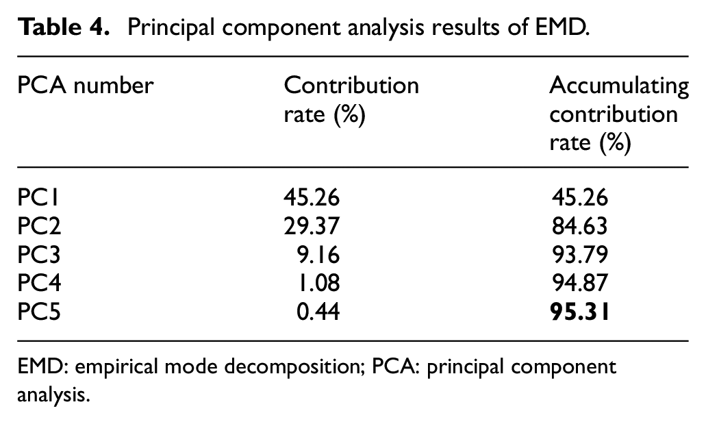
EMD: empirical mode decomposition; PCA: principal component analysis.

Pattern recognition

The principle of an artificial neural network is a mathematical model based on the structure of the brain’s synaptic connections, using computers to process information. An artificial neural network consists of a large number of unit nodes (neuron units) and the connection of weight coefficients between several units.^22,23 Each node unit represents a weight for the information passing through the connection, which is called neural network memory. This article selects a back-propogation (BP) neural network, which is a supervised neural network. Figure 9 shows the structure of the BP neural network. It contains an input layer, a hidden layer, and an output layer. The input of the network consists of the n principal components calculated as the main component, and the output is the bond failure mode. If the input is a position-off bonding, the network output vector is [0, 0], the wire breakage failure is [0, 1], the noncontact bonding is [1, 0], and the root peeling bond point is [1, 1].

Figure 9.

The structure of BP neural network.

A large amount of data training was carried out on the bonding samples, and 300 pairs of bonding samples (75 groups for each failure mode) were selected as validation data for testing. The WVD and EMD data are shown in Tables 5 and 6, respectively. Samples 1–4, 5–8, 25–28, and 297–300 represent position-off bonding, wire-bonding failure, noncontact bonding, and the root peeling bonding point, respectively.

Table 5.

Network output of the test sample.

Number	BPNN output	Accuracy	Number	BPNN output	Accuracy
1	[0.000,0.001]	True	25	[0.996, 0.006]	True
2	[−0.001, 0.012]	True	26	[0.993, −0.012]	True
3	[0.009, 0.603]	False	27	[1.003, 0.007]	True
4	[0.008, −0.003]	True	28	[1.001, 0.004]	True
5	[0.000, 1.020]	True
6	[−0.010, 0.965]	True	297	[1.004, 1.012]	True
7	[0.000, 1.008]	True	298	[0.173, −1.008]	False
8	[0.826, 1.000]	False	299	[1.049, 1.023]	True
			300	[−1.005, 0.964]	False

BPNN: back-propogation neural network.

Table 6.

Network output of the test sample.

Number	BPNN output	Accuracy	Number	BPNN output	Accuracy
1	[0.000, 0.001]	True	25	[0.991, 0.003]	True
2	[−0.001, 0.002]	True	26	[1.065,0.003]	True
3	[0.008, −0.033]	True	27	[0.0964, −0.007]	True
4	[0.011, −0.003]	True	28	[1.021, 0.004]	True
5	[0.000, 1.040]	True
6	[−0.010, 1.052]	True	297	[1.014, 0.912]	True
7	[0.004, 1.013]	True	298	[0.103, −0.008]	False
8	[0.019, 1.000]	True	299	[1.040, 1.073]	True
			300	[1.035, 0.958]	True

BPNN: back-propogation neural network.

Conclusion

This article aimed to detect the quality of the ultrasonic wire bonding by the joint time–frequency distribution and EMD methods. The average recognition accuracy of WVD was 78%. The position-off bonding recognition accuracy rate was approximately 76%, the wire breakage bonding recognition accuracy rate was 80%, the noncontact bonding recognition accuracy rate was 82%, and the accuracy rate of root peeling bonding point recognition was approximately 72%. From a statistical data point of view, the recognition accuracy rate based on the time–frequency distribution contour area bonding failure pattern recognition is acceptable. The average recognition accuracy of EMD was 93%. The position-off bonding recognition accuracy was approximately 93%, the wire breakage bonding recognition accuracy was 95%, the noncontact bonding recognition accuracy was 97%, and the accuracy rate of root peeling bonding point recognition was approximately 87%. The recognition accuracy of EMD is obviously higher than that of WVD. For high-precision bonding equipment, the bonding quality requirements are very strict, so the accuracy needs to be further improved. In a later stage, better feature extraction methods of ultrasonic electric signals can be used to further improve the recognition accuracy and reliability, which has certain research value.

Footnotes

Handling Editor: Francesc Pozo

Declaration of conflicting interests

The author(s) declared no potential conflicts of interest with respect to the research, authorship, and/or publication of this article.

Funding

The author(s) disclosed receipt of the following financial support for the research, authorship, and/or publication of this article: The work was supported by the basic scientific research fees of Zhejiang Ocean University (grant no. 2019JZ00004), the Provincial first-class discipline construction project—supported by young and middle-aged discipline leaders of Zhejiang Province, and Science and technology plan project of Zhoushan science and Technology Bureau (grant no. 2018C21014).

ORCID iD

Xin Chen

References

Liu

Tong

Wang

, et al. Challenges and developments of copper wire bonding technology. Microelectr Reliabil 2012; 52: 1092–1098.

Huang

Pan

YC.

Automated visual inspection in the semiconductor industry: a survey. Comp Ind 2015; 66: 1–10.

Zhao

, et al. Progress in ultrasonic bonding wire process and quality evaluation of bonding point. In: AOPC: optical sensing and imaging technology and applications, Beijing, China, 4-6 June 2017, p. 10462. Bellingham, WA: International Society for Optics and Photonics.

Schneider-Ramelow

Ehrhardt

The reliability of wire bonding using Ag and Al. Microelectr Reliabil 2016; 63: 336-341.

Wang

Ruan

Bai

, et al. Investigation on the bonding quality of GaN and Si wafers bonded with Mo/Au nano-layer in atmospheric air. Mater Sci Semicond Process 2020; 114: 105069.

Michaela

Petr

Jan

, et al. Characterization of bonding quality of a cold-sprayed deposit by laser resonant ultrasound spectroscopy. Ultrasonics 2020; 106: 106140.

Feng

Meng

Xie

, et al. Wire bonding quality monitoring via refining process of electrical signal from ultrasonic generator. Mech Syst Signal Process 2011; 25: 884–900

Mazloum-Nejadari

Khatibi

Czerny

, et al. Reliability of Cu wire bonds in microelectronic packages. Microelectr Reliabil 2017; 74: 147–154.

Khotanzad

Banerjee

Srinath

MD.

A vision system for inspection of ball bonds and 2-D profile of bonding wires in integrated circuits. IEEE Trans Semicond Manufact 1994; 7(4): 413–422.

10.

Koh

Lim

. Computer vision techniques for IC wire-bond height inspection. In: Automatic inspection and novel instrumentation, Singapore, 23 June 1997, pp. 11-21. Bellingham, WA: International Society for Optics and Photonics: 11–21.

11.

Meng

Feng

, et al. Simulation of displacement response of capillary and feature extraction for wire bonding process monitoring. In: ICMIT 2005: information systems and signal processing, Chongqing, China, 20-23 September 2005, p. 60411. Bellingham, WA: International Society for Optics and Photonics.

12.

Long

Han

, et al. Joint time-frequency analysis of capillary tip vibration in thermosonic wire bonding. In: Conference on high density microsystem design and packaging and component failure analysis, Shanghai, China, 27-29 June 2005. New York: IEEE.

13.

Zhong

Goh

KS.

Investigation of ultrasonic vibrations of wire-bonding capillaries. Microelectr J 2006; 37(2): 107–113.

14.

Mayer

Schwizer

Microelectronic bonding processes monitored by integrated sensors. Sensors Update 2002; 11(1): 219–227.

15.

Yoon

Eom

Lee

, et al. A capacitive micromachined ultrasonic transducer-based resonant sensor array for portable volatile organic compound detection with wireless systems. Sensors 2019; 19(6): 1401.

16.

Ghasemi

Abedi

Mokhtari

. Real-time method for resonant frequency detection and excitation frequency tuning for piezoelectric ultrasonic transducers. In: Australasian universities power engineering conference (AUPEC), Brisbane, QLD, Australia, 25-28 September 2016. New York: IEEE.

17.

Arjmand

Agyakwa

Corfield

, et al. Predicting lifetime of thick al wire bonds using signals obtained from ultrasonic generator. IEEE Trans Comp Pack Manufact Tech 2016; 6(5): 814–821.

18.

Yang

Zhang

Wen

, et al. Parameterised time-frequency analysis methods and their engineering applications: a review of recent advances. Mech Syst Signal Process 2019; 119: 182–221.

19.

Tsai

TN.

An adaptive diagnosis system for copper wire bonding process control and quality assessment in integrated circuit assembly. Int J Comp Integr Manufact 2013; 26: 513-526.

20.

Liu

Tang

On time-frequency domain feature extraction of wave signals for structural health monitoring. Measurement 2018; 114: 51–59.

21.

Mousavi

Taskhiri

Holloway

, et al. Feature extraction of wood-hole defects using empirical mode decomposition of ultrasonic signals. NDT&E Int 2020; 114: 102282 .

22.

Kontonatsios

Spencer

Matthew

, et al. Using a neural network-based feature extraction method to facilitate citation screening for systematic reviews. Expert Syst Appl 2020; 6: 10030.

23.