
Abstract
Power management in wireless sensor networks is very important due to the limited energy of batteries. Sensor nodes with harvesters can extract energy from environmental sources as supplemental energy to break this limitation. In a clustered solar-powered sensor network where nodes in the network are grouped into clusters, data collected by cluster members are sent to their cluster head and finally transmitted to the base station. The goal of the whole network is to maintain an energy neutrality state and to maximize the effective data throughput of the network. This article proposes an adaptive power manager based on cooperative reinforcement learning methods for the solar-powered wireless sensor networks to keep harvested energy more balanced among the whole clustered network. The cooperative strategy of Q-learning and SARSA(λ) is applied in this multi-agent environment based on the node residual energy, the predicted harvested energy for the next time slot, and cluster head energy information. The node takes action accordingly to adjust its operating duty cycle. Experiments show that cooperative reinforcement learning methods can achieve the overall goal of maximizing network throughput and cooperative approaches outperform tuned static and non-cooperative approaches in clustered wireless sensor network applications. Experiments also show that the approach is effective in response to changes in the environment, changes in its parameters, and application-level quality of service requirements.
Keywords
Introduction
A key challenge that limits the applications of wireless sensor networks (WSNs) is the battery lifetime generated by the restricted energy storage of each sensor node. Energy harvesting wireless sensor networks (EH-WSNs) can extract energy from environmental sources as supplemental energy to break this limitation.1,2 The latest developments in energy harvesting technology can greatly extend the sensor network lifetime and may run permanently without replacing sensor batteries strenuously which is even not feasible in some cases. The energy that can be harvested often varies with time and uncertainty. Consistent with the node’s energy collection and node workload, the use of adaptive energy management strategies to improve energy utilization can thereby improve the system performance and system sustainable operations. 3 At the same time, the energy harvesting efficiency of energy harvesting batteries is affected by weather, climate, and location. Bandwidth is also an important challenge. These limitations require sensor networks to be able to adapt to the changing environment and effectively use the available energy. Besides, in practical applications, WSNs need to adapt to changes in device parameters and system degradation to dynamically meet application-level quality of service (QoS) requirements (such as network delay, data throughput, and energy consumption).4,5
To solve the above problems, approaches in developing WSN protocols with low power consumption, high performance, and low latency, such as medium access control (MAC) protocol, routing protocols, and data aggregation methods, are developed. 6 The advantage of these solutions is that the system’s low power consumption is achieved, but the nodes are difficult to achieve long-term operation. Even if solar cells are used as energy sources, the system cannot adapt to changes in utilizing the harvested energy as much as possible. The node cannot either adjust automatically the duty cycle and information transmission rate to obtain optimal performance. Due to the dynamic nature of energy harvesting resources in WSNs, as well as the variation of network environment such as different network topology, node residual energy, and energy consumption, the static approach apparently cannot be good enough to solve the problems faced by EH-WSNs. Reinforcement Learning (RL) 7 is a learning method aiming at maximizing the cumulative reward of system behavior from the environment, which is suitable for adaptive energy management strategies. RL is mainly divided into value-based methods and policy-based methods, as well as the combined methods known as Actor-Critic methods. RL algorithms have been practically used in many fields, and they also have certain applications in energy management in the Internet of things (IoT). Based on the combination of its learning and the interaction of the environment, the agent can react to the changes in the changing environment to improve the performance of WSNs. 8
A general RL model consists of a finite state space

The environment’s response to this action is to change the state of the agent to a new state

where
In a cooperative way of RL, an agent interacts with other agents in the same environment. The rewards and actions’ information could be shared in different strategies among these agents. For example, an agent changes from state
This article proposes cooperative reinforcement learning (CRL) methods, specifically Q-learning and SARSA(λ), for adaptive energy management of EH-WSNs. CRL methods are used to achieve automatic energy management in IoT nodes in a clustered EH-WSN. The reward function is designed for maximizing the amount of valid data that the sink node finally received during a whole day, and minimizing the distance that the node leaves the energy neutrality state. The adjustable duty cycle sensor nodes of the whole network are grouped into clusters. Data collected by cluster members (CMs) are transmitted to their cluster heads (CHs) and finally received by the base station (BS). The goal of this network is to maintain an energy neutrality state and maximize the effective data collection of the BS. In reality, a WSN also needs to dynamically meet application-level QoS requirements, that is, to adjust its own operating state according to changes in the deployed environment. The agents share their CH energy information cooperatively within clusters. A series of simulations was conducted to explore the effect of our approaches on network performance compared to traditional approaches and other RL methods. Simulations show the adaptive power manager can ensure better network performance and avoid node energy depletion.
The main contributions of our work are listed as follows:
An adaptive power manager in EH-WSNs by CRL methods is proposed to increase the network throughput by sharing the information between sensor nodes in one cluster, such as residual battery energy and harvesting energy. In cooperative Q-learning and SARSA(λ) algorithms, each agent learns from the environment and their CH. It helps the nodes to learn to select the proper transmission rate under the uneven clustering network to maximize the network throughput.
The impact of the environmental parameters regarding different initial node energy, transmission power, and the number of sensor nodes in the field is explored.
Tuned static policy, stochastic policy, and genetic algorithms (GAs) are compared with the proposed algorithm which successfully provides better network QoSs.
The rest of this article is organized as follows. Section “Related work” presents a brief literature overview on EH-WSNs and RL. Section “System model” gives the whole framework of the system model. Section “CRL model” describes our CRL approaches for the energy manager to adaptively adjust the transmission rate in EH-WSNs. The experimental results and discussion are presented in Section “Simulation and results.” Section “Conclusion” is the conclusion of this article.
Related work
This section gives a brief overview of clustered EH-WSN and RL applications in power management of IoT.
Cluster-based EH-WSNs
Clustering routing protocols of WSNs have been extensively studied in the literature. They are represented by the low-energy adaptive clustering hierarchy (LEACH) 9 and its following improved algorithms. Their main goals are to achieve energy balance among the whole networks. However, these protocols may lead to the “hot spot” problem in WSNs, 10 that is, the nodes nearing the BS die faster than nodes far from the BS. Uneven clustering algorithm could solve part of this problem. The energy efficient uneven clustering (EEUC) algorithm 11 determines the uneven competition radius according to the distance between the nodes and the BS, so that the size of clusters close to the BS is smaller, saving energy for communication and transmission between clusters. Moreover, in the selection of the relay node, the remaining energy of the node and the distance from the CH to the BS are comprehensively considered. Considering the balancing the whole network energy, Peng and Low 12 proposed a routing protocol based on CH groups, in which CH group members take turns to balance CH energy consumption.
Some works have been done on maximizing network transmission information in WSNs and EH-WSNs, but more investigations under different protocols need to be explored more thoroughly. Wang et al. 13 investigated the mathematical formula to get the optimal transmitting power of nodes and the algorithm for selecting the CH to maximize the data gathering in WSNs. Mehrabi and Kim 14 introduced a mixed-integer linear programming (MILP) optimization model for maximizing network throughput in EH-WSNs. An uneven clustering protocol in solar-powered WSN is proposed in our previous work to maximizing the network throughput with fixed data rate in each node. 15
RL applied in power management
RL algorithms can learn optimal policy by interacting with an environment based on the reward. Value-based approach, such as Q-learning and SARSA, and the policy-based approach, such as proximal policy optimization (PPO) 16 using a neural network as a function approximator have been widely used in power management in IoT applications. An adaptive power manager is presented in Shresthamali et al. 8 to adjust duty cycles in solar energy harvesting sensor nodes using the SARSA(λ) method to ensure optimal network performance without draining its battery. It is evaluated at the end of each episode which is believed to achieve the ENO-Max objective better compared to traditional methods. The paper considers the factors on climatic factors and battery degradation. Ortiz et al. 17 proposed methods using RL optimization to achieve energy neutrality for power management. The reward function is based on the distance from the energy neutrality state and the remaining battery of the node. Although there may be a more general formula, this objective is a good rewarding strategy that indicates a certain state or action advantageous, rather than how to achieve the goal. We also use the same metric as part of state evaluation to determine rewards. Aoudia et al. 18 proposed an energy manager to maximize the throughput in a two-hop energy harvesting wireless network. SARSA is used to solve the problem in the whole network. Hsu et al. 19 proposed an RL approach named as RLMan as an energy manager according to the current remaining energy level and proved it more robust to the node consumption variation. Hsu et al. 20 presented an RL-based power manager by a Q-learning algorithm and trained the node to select duty cycles dynamically. Their reward function is energy neutrality state which is the distance from energy neutrality state to energy storage level and the throughput requirements. Rioual et al. 21 explored different reward functions to find the most appropriate variables in these functions to achieve the proposed performance. Experimental results from comparing the different functions present the effect of reward functions could result in different energy consumption. Given uncertain energy availability, Fraternali et al. 22 used RL algorithms to maximize the sample rate with available harvested energy. Most of the previous works use RL in regulating one single node duty cycles dynamically in IoT, without considering interactions between nodes affecting the network performance.
Multi-agent reinforcement learning (MARL) is a system where several agents interact in the same environment. The multi-agent environment represents as
Each agent makes certain actions at each time step and works together with other agents to achieve the goals. Due to the complexity of the MARL environment and the characteristics of multi-agent collaboration, the complexity of training multi-agents is relatively high, and most MARL problems are classified as NP-Hard problems. 23 which are difficult to find the solution algorithm of polynomial time complexity. The factors that need to be considered when modeling MARL systems include (1) centralized or decentralized control, (2) a fully or partially observable environment, and (3) a cooperative or competitive environment. In the centralized control mode, the centralized controller is responsible for each agent action in each time step. However, in a decentralized system, each agent’s behavior is determined by itself. Moreover, agents can cooperate to achieve common goals or may compete with each other to maximize their rewards. Under different circumstances, an agent may access all the information of other agents, or each agent may only observe its local information.
In the problem of cooperative environment, if an agent can fully observe the environment, each agent

where
Although the MARL method has been successful in practical applications, MARL has the nature of multi-agent combination problem, that is, its complexity will increase exponentially with the number of agents
There are several works in which the authors used CRL methods to optimize the performance of power management. Khan and Rinner 31 proposed a CRL method for determining and scheduling tasks based on its behavior and neighboring nodes’ information. Therefore, application performance and energy achieve a better trade-off. Emre et al. 32 introduced the so-called cooperative Q method which makes radios learn and adapt to their environment by sharing their information. Its proposal aimed to maximize energy efficiency while ensuring buffer occupancy below the predetermined level. Wu et al. 33 proposed a cooperative Q-learning method to investigate the energy management approach to optimize the network throughput. The network works on a preset routing protocol where the relay node receives data packets from the previous node and then transmits it to the next one. The whole process repeats until the data are finally sent to the BS successfully. A node regulates its duty cycle according to its neighbor’s energy information. Simulations show that their proposed scheme can work effectively to satisfy the network performance requirements. However, no previous research works have investigated the algorithms in a clustered WSNs where energy has already been balanced and the optimization of the duty cycle has more challenges in this environment.
System model
Figure 1 shows an overview of our system model and energy management approach. The adaptive energy manager uses CRL to monitor and regulate their duty cycles to keep the nodes in an energy neutral state. This is a typical clustered EH-WSN which has a BS and sensor nodes randomly located in the field. Each sensor node consists of energy harvesting equipment (solar panel) to complement energy, an energy buffer (supercapacitor), and a power manager for each node (agent). They are divided into clusters periodically. The CHs of clusters are rotated throughout the system life cycle, for preventing them from replenish their limited energy. Once the CHs lose all the energy, they are no longer operational and all the CMs belonging to the cluster lose their communication capabilities. All the CHs collect data sent by the CMs within their clusters, then aggregate and forward these data to the BS. We assume that the BS can access an unlimited amount of energy. The agent can adjust its duty cycle according to the node and environmental state. To achieve the maximum overall throughput during a period of operation time (usually a whole day), we also utilize the periodical predicted energy information of each node from the energy predictor proposed in Ge et al. 34
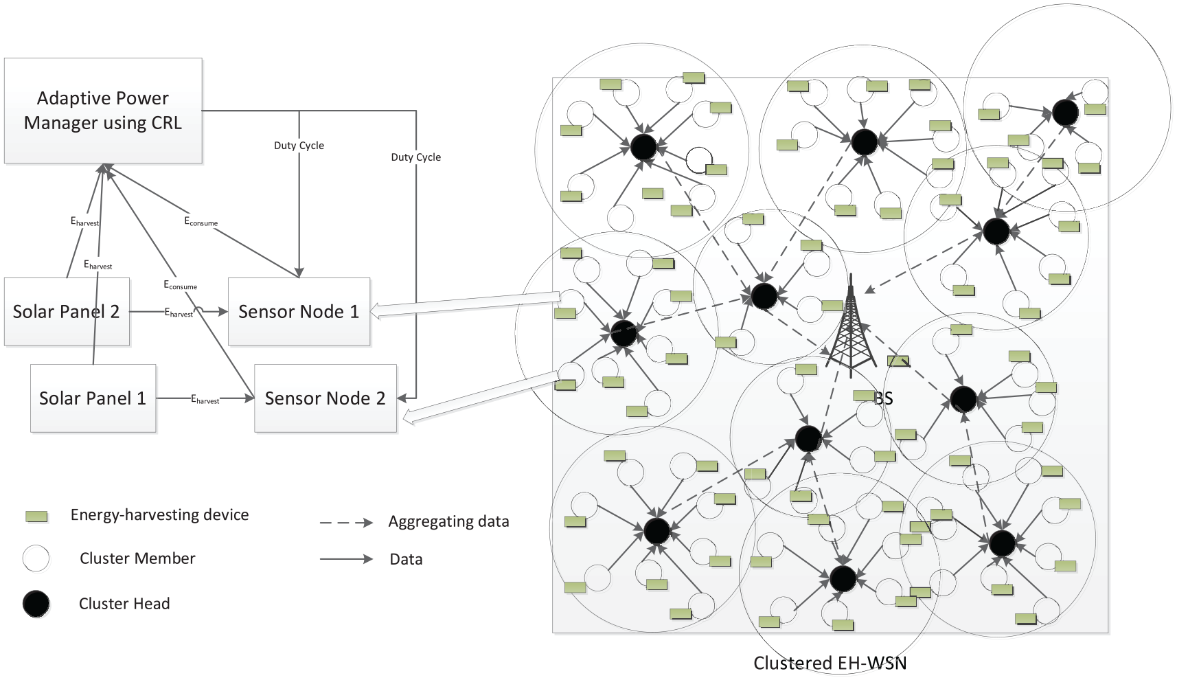
System model and our approach.
The uneven clustering protocol is deployed in our system. For each node
Step 1. Tentative CH selection: at the beginning of each round, nodes are randomly selected as tentative CHs, if
Step 2. CH competition: for any tentative
where
Step 3. Cluster formation: each node calculates the distance to all the CHs and joins the closest CH.
The energy consumption model from LEACH 7 is adopted in the network, including energy consumed during transmission, reception of packets, and data dissemination. The details are described in section “Simulation and results.”
CRL model
Framework of CRL
Our framework of CRL defines a group of cooperative sensor nodes under the EH-WSN environment where action and state space are modeled. Agents are trained in each round of cluster formation. Each node harvests a certain amount of energy in one time slot. The current state of each node consists of the residual energy, the solar energy that could be harvested in the next time slot, and its CH residual energy. At the end of each round, the agent will receive some rewards for evaluating its behavior and upgrading its strategy (Q-table). The agent keeps taking a series of actions and traverses the alternating state until the end of the episode. The state definition, the action space, and the reward scheme are described below.
Environment
In the EH-WSN, the whole network tries to achieve energy balance and high network throughput. Sensor nodes can supplement energy from their solar panel. In each round, clusters are formed periodically. Each CM transmits the data to its CH, and then the CH will aggregate the data from its CMs and then send all the data to the BS. For energy efficiency, the energy manager would prevent the node from depletion completely. Each node will determine the transmission rate to be set based on the predicted energy and the remaining energy for the next time slot.
Agent
The agent of each node communicates with the environment and takes the power management action. The agent is trained by a series of episodes. Each episode has 24 hours and 10 times of cluster reformation per hour, therefore there are 240 rounds per episode. The node transmission process of each round includes the information exchanging stage and data transmission stage. In each round of information exchange stage, each agent in the cluster can receive CH information, including energy information.
Action
The action space
State
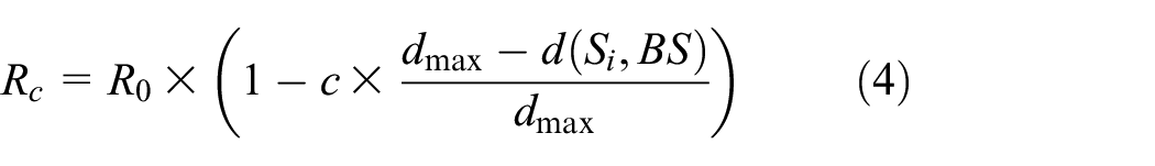
In order to achieve long-term stability of the network and high transmission of information, the nodes in the energy harvesting WSN need to determine the data transmission rate based on their own remaining energy and the energy that can be harvested in the next cycle, and it is related to the energy level of the next relay node. The current state of the energy level of the non-CH node becomes an important factor to determine the data transmission rate. The observation state of each node consists of three observations in equation (5)


where

where
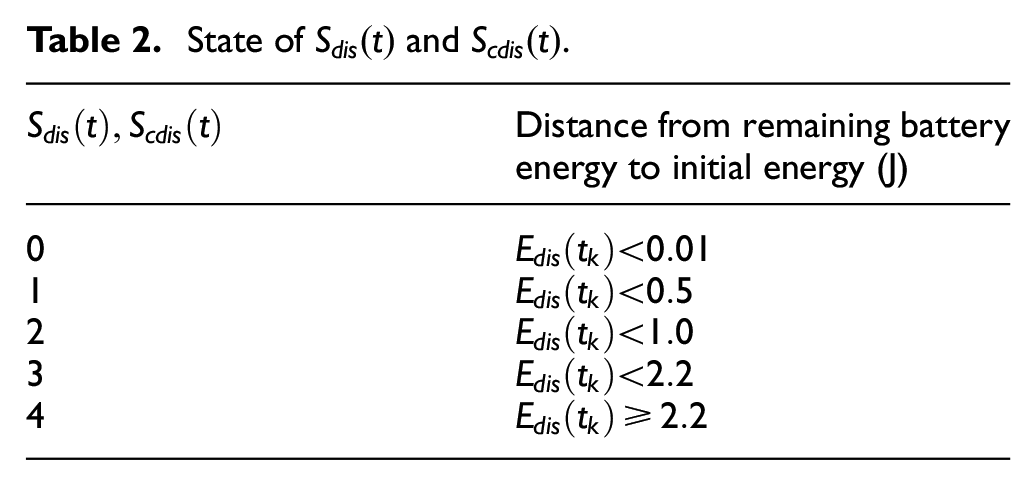
State of

State of
Reward
The objective function of our system is to maximize the throughput and balance the energy. The goal of the system is to send as much data as possible under limited energy resources while keeping the node in an energy neutrality state and avoiding less number of energy depletion of nodes. The reward calculated in equation (8) is then designed for achieving this goal

Cooperative Q-learning algorithm
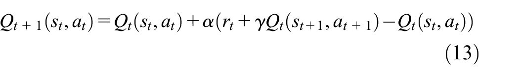
Q-learning is a classic value-based off-policy RL algorithm. It is expected that taking action
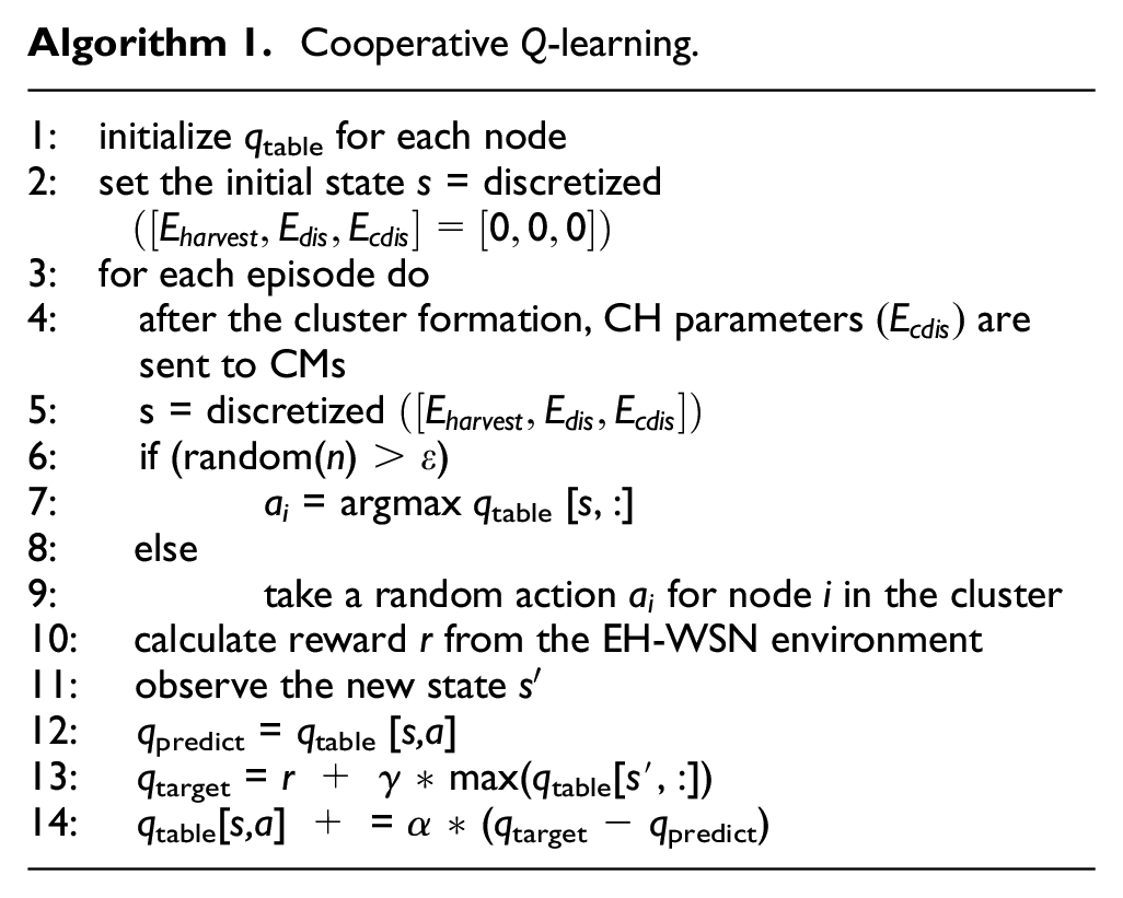
Algorithm 1 illustrates the steps of the cooperative Q-learning algorithm. After initializing the qtable of each node to a zero matrix (line 1), the node state (i.e. residual energy, CH residual energy, and predicted energy) is discretized and received by the agent (line 2). The algorithm then goes into a while loop. Each CH sends its parameters to it CMs (line 4). According to its state (line 5), each node starts to select an action (line 4) which follows the ϵ-greedy policy (line 6–9). Then, each node in the cluster changes its transmission rate and the reward is returned accordingly (line 10). The next state of each node is observed in each round (line 11). The Q-table of each agent is updated separately according to the state, the next state, and selected action (line 12–14). qpredict is the q-value of taking action
Computational complexity analysis
Considering the computational complexity of each iteration in the MARL environment, since each node maintains its own q-table, the highest computing burden is attributed to the state–action search of the q-table and the update of the corresponding state. Algorithm 1 uses the ϵ-greedy strategy for each agent node to select actions in a certain joint state. The time complexity for searching the node’s q-table and updating q-table is
Convergence analysis
The Q-learning algorithm was first proposed in the literature. 35 It is a major breakthrough in RL because this is the first RL algorithm that guarantees to converge to the optimal strategy. Its convergence is proved in the literature. 36 In a certain Markov decision process (MDP), the Q-learning algorithm can be equivalently defined as

The individual Q-learning algorithm is known to converge to the optimal
It is required that the sum of learning rates must diverge, but the sum of squares must converge as shown in equation (10)

Each state–action must be accessed unlimited times: each action in each state must be selected by the strategy with non-zero probability, that is,
Through the previous analysis, the value function

Proposition 1
For the deterministic MDP model

where
Proof
t ↝ t + 1: at any time t, all agents take action
When
When

Assume that equation (12) holds at time step t, then

Since

From equation (9), we have

Because the Q-table is monotonically increasing

Therefore, equation (12) holds at
Cooperative SARSA(λ) algorithm
SARSA algorithm is an on-policy algorithm which is a temporal difference learning approach to solve RL control problems. Given five elements of an RL environment: state space S, action space A, instant reward R, attenuation factor γ, exploration rate
where
SARSA(λ) algorithm is the alternation of standard SARSA to improve the algorithm. After each action is taken in SARSA, only the previous step is updated which is SARSA (0) while SARSA(λ) can update the step before the reward by having the trace decay factor

Comparing with SARSA, it has an additional matrix E[s,a] (eligibility traces) in the algorithm which is used to save the contribution of each step in the path to the subsequent reward which is defined as

SARSA(λ) can learn the optimal strategy more quickly and effectively. Because the action
We apply cooperative SARSA(λ) for adaptive power management in EH-WSNs. Each node has a common goal, which is to maximize the network throughput. In time period


Algorithm 2 describes the steps of the cooperative SARSA(λ) algorithm. After initializing the qtable of each node to a zero matrix (line 1), the state of each node (node residual energy, its CH residual energy, and predicted energy information) is discretized (line 2). After clustering formation, the CH information is sent to each CM (line 4). Each node in the cluster selects its own action according to its q-table and calculates the reward accordingly (line 8). In each round, the next state of each node is observed (line 9). According to the current state, the next state, and the selection action, the q-table and the eligibility trace matrix will be updated individually (lines 10–15).
Similar to the collaborative Q-learning method, the collaborative SARSA algorithm considers the computational complexity of each iteration. The complexity of energy management policy based on clustered EH-WSNs is independent of the number of nodes
In SARSA, when searching for the best solution, the strategy π is updated. Evidence shows that select the action
Simulation and results
A clustered EH-WSN network environment is carried out on Python. The simulation environment constitutes the system environment of sensor nodes that continuously communicate with the adaptive energy manager implemented in the CRL algorithm. Agents select actions (data transmission rate) to adjust the nodes’ state in order to optimize network data transmission. In the following sections, energy data resources, the model configuration of the network, and case studies are described in detail.
Energy source
The data to simulate the harvested solar energy are retrieved from the US Department of Energy, National Solar Radiation Database 39 which contains historical solar data with a 1-h sample rate and statistics results in more than 1000 locations of the United States. Data from different locations, including Michigan, Alabama, and Nevada, are used in the experiments in order to compare the performance of RL methods. Figure 2 shows 7 continuous days of global horizontal solar radiation profile in a site of Alabama in 2008. It shows different amounts of hourly energy available for harvesting under the different weather conditions where January 17 and 18 have obvious lower harvesting resources available than the other 5 days.

Solar radiation profile in Alabama 2008.
EH-WSN clustering and energy-related parameters
In the sensor network field area, the example of a clustered solar power network with 60 sensor nodes is depicted in Figure 3. The field is a square with the length of 200 m. Each node uses a solar panel device to complement energy. The stationary BS with the “X” shape marker in our system model is deployed in the middle of the WSN field by which a better performance can be achieved. 40 The BS could get access to an unlimited amount of energy and have strong computational power. All the nodes are grouped periodically into different clusters by the same color. Each cluster is composed of a CH indicated by a triangle marker and some CMs with dot markers. Data are sent by the CMs to their CHs, then aggregated and forwarded to the BS. Section “System model” describes the steps of the uneven cluster formation algorithm in detail. Figure 3(a) and (b) forms five different clusters, respectively, in different rounds. These two graphs show different clustering methods based on the same distribution of nodes, including the number of nodes and position coordinates. The positions of the CHs have changed as the CH rotation of the network during the initialization phase of each round, which is conducive to balancing energy load and prolonging the network life.
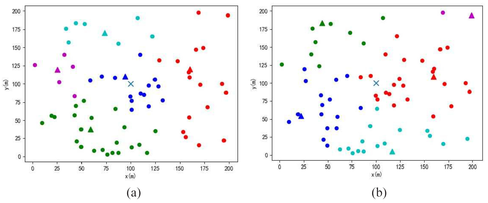
Examples of EH-WSNs: (a) one formation of five clusters and (b) another formation of five clusters.
The energy consumed in the simulation system is calculated according to the energy consumption model in Heinzelman et al.
9
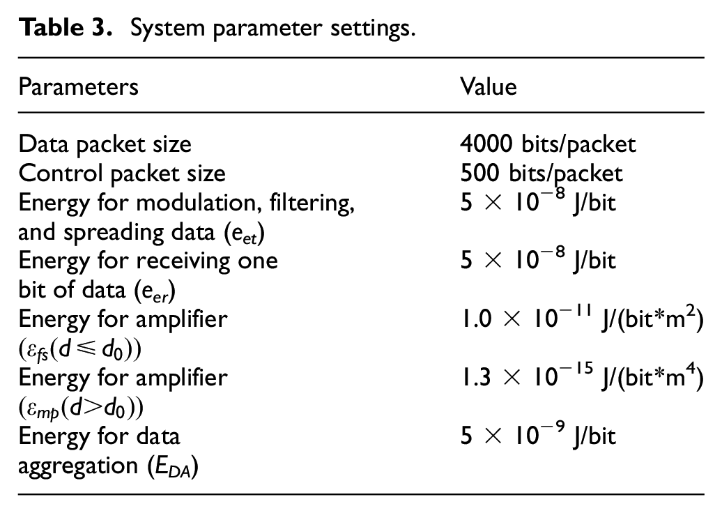
Assuming that the model is ideal, energy consumption—such as data acquisition and data storage—is constant. Besides it is assumed that there is no static energy consumption which can be set to 0 in the simulation, and the energy consumed by the battery itself is ignored. For simplicity, assume it is an ideal battery. The initial battery size of the sensor node is initialized as 0.5 J. For the other parameters in the system: the wireless sensor deployment area is a 200 m × 200 m rectangle and the BS is located at the middle of the area with the coordinates (100 m, 100 m). The total number of sensors is 20, 40, and 60, respectively, in different cases. The probability of the sensor being selected as the CH is 0.2. The size of the control packet for communication between the nodes is 500 bits/packet, the size of the data packet is 4000 bits/packet,
System parameter settings.
Tuning parameters
The system has several parameters to be set including clustering parameters (parameters to control the cluster size
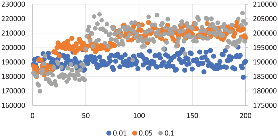
The learning rate α determines how fast the model moves to the optimal value and is a trade-off between the previous and current learning results. Too low value of α may cause agents to only care about the previous knowledge and cannot accumulate new rewards. Too high value of α may cause excessive fluctuations of Q-values during training. Numerous studies start commonly with a high learning rate so that learning results can change quickly, and then over time, the learning rate is reduced. Under our environment, Figure 4 shows when α is 0.01, there is no improvement within 200 iterations; when α is 0.05, the higher performance of the network is achieved; when α is 0.1, the system also converges faster; when α is set to gradually decrease from 0.1 to 0.05, the experimental performance is similar to when α is set to 0.1.
Different learning rate comparison.
The discount factor γ accesses the impact of future reward value compared to immediate rewards which is usually set between 0 and 1. When the discount factor γ is 0, only the current reward is considered, adopting a short-sighted strategy. The larger the value of γ, the more future benefits we have considered the value generated by the current behavior. If the value of γ is too large, the consideration is too long-sighted, even beyond the range that the current behavior can influence which will affect the convergence of the algorithm. Empirical experiments show how the discount factor impacts the training performance of the whole network throughput. When γ is higher than 0.9, the performance of the system varies rapidly during the process. When γ is less than 0.7, the network throughput is comparatively low and difficult to achieve comparatively high network QoS. Considering these results, γ is set as 0.9.
When the agent chooses actions based on its own q-table, it uses the ϵ-greedy algorithm. If ϵ = 0, a completely greedy method means the highest q-value is always selected among all q-values in a specific state, which may lead to a local optimal state. The randomness of ϵ is necessary for exploration. In the experiment, ϵ is set to 0.1 which means the agent chooses a random action with a probability of 0.1.
The trace decay parameter λ in eligibility traces in SARSA(λ) controls how eligibility decays over time. Through experiments, when λ increases, SARSA(λ) with a higher λ converges quickly at the first stage of training to than with a lower λ. But when λ is 0.9, some lower performance is observed. In order to balance the trade-off between good performance and convergence, the trace decay λ is regulated as 0.8.
Results and discussions
The performance of the EH-WSN network is measured by the number of data packets successfully transmitted to the BS of the network in one whole day. Distributions of nodes of the networks are generated randomly in each simulation.
Performance evaluation
Figure 5(a) and (b) shows the network throughput of Q-learning and SARSA(λ) algorithm results, respectively, in its optimal policy when all 60 nodes in the field are trained over 700 iterations. It is obvious that the total number of data packets transmitted by the network increases as the network is trained by the CRL, and then the data oscillate around 170,000 packets to 218,000 packets. This shows that in the current network configuration, the optimal performance of the strategy is 218,000 packets. Cooperative Q-learning and SARSA(λ) achieve similar performance. Figure 6 shows the node transmission rate changes of a node in one iteration both at the beginning of Q-learning training and after 500 iterations. The supplement energy charges the nodes every 4 h. Figure 6(b) and (d) shows the battery residual energy at the beginning of the training and 500th iteration, respectively. At the beginning of the training shown in Figure 6(a), the transmission rate is quite random and after 500 iterations’ training, the node is trained to set at 22 packets/round since the harvested energy is abundant as shown in Figure 6(c). The nodes could operate continually by the stored energy at night time (around round# 180 to 240).
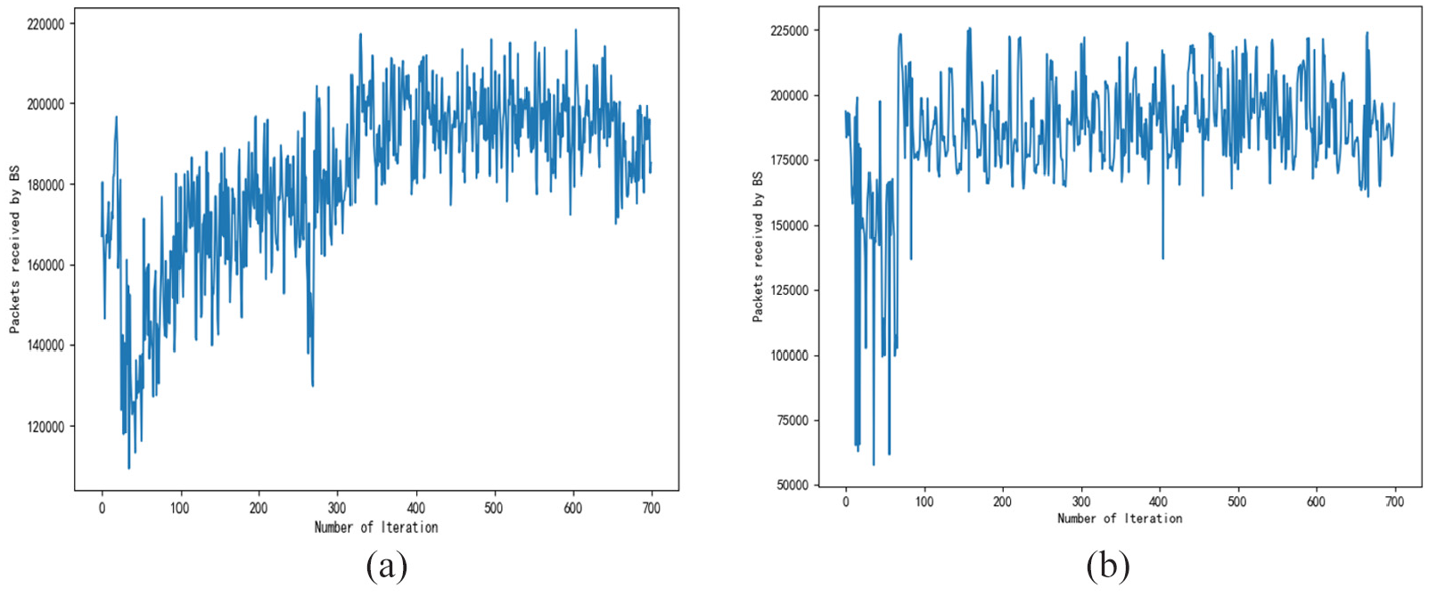
CRL iterations: (a) cooperative Q-learning and (b) cooperative SARSA(λ).
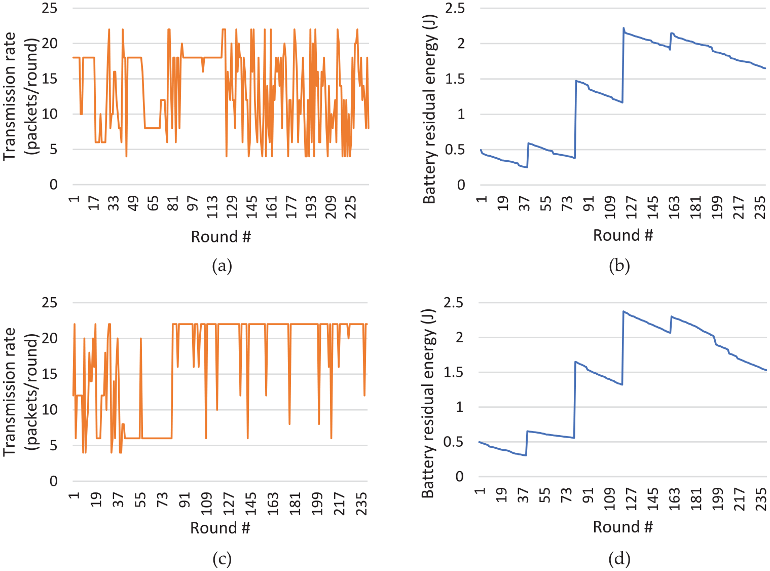
Transmission rate and battery energy changes of cooperative Q-learning: (a) transmission rate profile at the beginning of the training, (b) battery residual energy at the beginning of the training, (c) transmission rate profile at 500th iteration, and (d) battery residual energy at 500th iteration.
Comparison with static policy
Under the static transmission rate, the network data transmission performance is shown in Figure 7 which indicates that the performance of the network is sensitive to the predefined data transmission rate, that is, the network performance at different data transmission rates varies greatly. Figure 7(a)–(d) shows under static transmission rate when the transmission rate is set as 8, 12, 16, and 20 packets per round. In Figure 7(d), the network performance of this certain case has a high deviation under different clustering formation and has little chance to have good network performance since the energy cannot maintain the transmission rate as high as 20 packets per round. According to Figure 8(a), under static data transmission, 18 packets/round for each node are optimal in the current configuration. When the transmission rate is less than 18 packets/round, the node energy is relatively abundant, and the performance of the network increases as the rate increases. When the transmission rate is greater than 18 packets/round, the high data transmission rate makes the node energy consumption too quick, causing some nodes to be exhausted and become dead. Thus, the network performance declines dramatically under 20 packets/round. Figure 8(b) shows the same trend that the number of dead nodes increases rapidly especially when the transmission rate is above 18 packets/round. The performance of the network depends on the specific network configuration (including system parameters) with the optimal transmission rate. However, it is not always able to know the optimal transmission rate for each network configuration, and tracking changes in network parameters and environments is particularly difficult in the case of constantly changing network parameters and environments which limits the performance of the whole network. The cooperative Q-learning strategy is obviously better than the best performance of the optimal static strategy with 213,000 packets. Considering the adaptability of the strategy to the environment and the optimal strategy, using manually configuration is not applicable, so the network may not be able to run at the optimal rate. To compare different approaches under different network environments, more experiments have been done on cooperative Q-learning and SARSA(λ).

Network throughput by static transmission rate: (a) packet rate = 8, (b) packet rate = 12, (c) packet rate = 16, and (d) packet rate = 20.

Network performance under different transmission rates: (a) network throughput under different constant transmission rates and (b) number of dead nodes under different constant transmission rates.
Comparison with stochastic policy and GA
To evaluate the performance of the proposed algorithm, a stochastic policy was also implemented. A stochastic policy simply enumerates every possible combination in the solution space, evaluating each and keeping the record for the best solution to date. Table 4 shows one possible solution for one round of energy management in EH-WSNs. However, the efficiency of stochastic policy is extremely low. The solution is represented as a two-dimensional array with height as node dimension and width as time slot dimension. Each cell in the array is assigned one value from the set of {4, 6, 8, 10, 12, 14, 16, 18, 20, 22, 24, 26}. If there are 60 nodes in the field, a total number of 1260*240 different combinations. Within 500 iterations and 10 different distributions for 20, 40, and 60 nodes in the field, the performance of random search and collaborative Q-learning is shown in Table 5. The results show that in one case of 40 nodes, the performance of collaborative Q-learning is close to random search. In most situations, collaborative Q-learning outperforms random search.
Possible solution.

Comparison with random search.

GA is inspired by natural science to simulate the evolution of biological populations. After the initialization of population, evolution, selection, mutation, and crossover operations are implemented on the population to produce a new generation that is expected to be closer to the global optimal solution. The evolution continues until a certain step ends or some criteria are met. Algorithm steps include as follows:
Select the initial population.
Evaluate the fitness of individuals in the population.
Select proportionally to produce the next population.
Change the population.
Judge the stop condition and return to the second step if not satisfied.
Our initial population of individuals as shown in Table 4 is chosen randomly. Individual fitness of the population is the number of packets sent to the BS successfully. The next generation is selected proportionally. Individuals with high adaptability (a bigger number of packets transmitted) will be selected in a higher proportion, and other individuals with low adaptability will be selected at a lower proportion. In this way, a new population is generated. Crossover and mutation are also applied to modify the individuals and generate new individuals. The simulation is implemented using the GA package for Python, named geneticalgorithm. 42
Table 6 shows GA performance in different situations. Comparatively, within limited iterations, the GA cannot achieve good performance compared to CRL. Under the situation of 60 nodes, the GA approach with 500 generations achieves the best performance 168,780 and collaborative Q-learning can achieve the best performance of 221,123. In GAs, each agent does not have a dynamic learning process and the whole learning process evolves on the whole population. Therefore, GAs are only suitable for problems such as the strategy space is small enough. The evolutionary algorithm also ignores that policy is actually a mapping from state to action and does not learn features from the interaction with the environment. Therefore, RL can generally find the right policy more effectively. As shown in Figure 9, the collaborative Q-learning policy can achieve better performance over random search and GA under 500 iterations. The GA approach takes much more computation burden since there are dozens to hundreds of individuals in each generation.
Genetic algorithm performance.


Comparison of performance by different policy.
Adaption to parameter change
Adaption to battery degradation
In order to simulate the battery degradation of a sensor node, the initial energy of the node battery is reduced to 80%, 60%, and 40% of the original battery capacity. The cooperative Q-learning and SARSA(λ) results are shown in Figures 10 and 11. In this case, the cooperative Q-learning and cooperative SARSA(λ) strategy have similar behavior and can still adapt to changes, and their network throughput performance is better than static transmission by 16.6%–30.1%. In terms of the number of dead nodes, there are 60 nodes in the network. If one node in each round is dead in one moment, the number of dead nodes is counted as 1. There are 240 rounds in each iteration (24 h). In Figure 9, the number of dead nodes refers to the number of all dead nodes in 240 rounds (24 h) which are between 1500 and 3000. Cooperative Q-learning and cooperative SARSA(λ) have fewer dead nodes in every 24 h than the static method by 21.0%–45.9%.

Network throughput under battery degradation.

Total number of dead nodes under battery degradation.
Adaption to changes in equipment parameters
The sensor nodes in IoT need to experience changes in equipment parameters, such as equipment energy efficiency. This experiment is designed for the change of node energy efficiency. In order to simulate the change of device parameters, the power consumption of the node is changed by 125%, 100%, 75%, 50%, and 25%. The results of the network performance under different equipment parameters are shown in Figures 12 and 13. The results reveal that cooperative Q-learning and cooperative SARSA(λ) are still adaptable and have better performance than the tuned static algorithm. When the original power consumption is increased to 125%, the network throughput rate in all cases is reduced, but the information transmission rate is still higher than that of the static method. At 6.8% and 11.8%, when the power consumption is reduced to 75%, 50%, and 25%, cooperative Q-learning and cooperative SARSA(λ) methods are still higher than the static method by 5.5%–18.5%. In terms of the number of dead nodes, 60 nodes are randomly distributed in the field. There are 240 rounds of data transmission in each iteration (24 h) and the number of dead nodes in each round is recorded as 1. The number of dead nodes refers to the number of all dead nodes in 240 rounds. From Figure 13, cooperative Q-learning and cooperative SARSA(λ) have fewer dead nodes in each iteration than the static method by 8.9%–37.3%, especially in the two high energy consumption situations of 125% and 100%. When the energy consumption is 100%, cooperative Q-learning and cooperative SARSA(λ) methods are 29.7% and 27.0% higher than the static method, respectively. When the energy consumption is 125%, cooperative Q-learning and cooperative SARSA(λ) are respectively higher than the static method 37.3% and 34.6%.

Network throughput equipment parameter changes.

Total number of dead nodes under equipment parameter changes.
Adaption to changes in different field node densities
Finally, different densities of network sensor deployment are considered in the field. The density of sensor nodes may affect the clustering and the transmission distance between the nodes. Figure 14 shows the comparison results of constant transmission rate policy, cooperative Q-learning, and cooperative SARSA(λ) when the sensor nodes in a field are 20, 40, and 60, respectively. The cooperative Q-learning and SARSA(λ) algorithms are averagely better than the constant transmission rate policy in the network throughput.

Comparison of constant transmission rate policy.
Conclusion
The adaptive power management system of this article uses cooperative Q-learning and SARSA(λ) algorithm to optimize the data transmission rate of EH-WSNs, rather than relying on the manual configuration of the node transmission rate. This is the first application of CRL to adaptively manage the transmission rate of nodes in clustered solar-powered WSNs. Experiments show that the network with CRL power management policy can adapt itself to environmental changes, and sensor nodes can determine the data transmission rate according to their own residual electricity and collectible energy. Compared with the general network, the data transmission performance of the optimized network has been improved. At the same time, the network can adapt to the changes of equipment parameters, battery degradation, and node density changes, which ensures the reliability and stability of networks in the application and enhances the practical application performance of the network. Although this article focuses on maximizing information transmission, these methods are applicable to various situations of WSNs and a wider range of IoT applications by designing new reward function.
The complexity and convergence of the proposed algorithms are analyzed. Algorithms such as cooperative Q-learning and SARSA based on discrete table values have a limit on the number of states which are not suitable for continuous state modeling. Future work will explore using function approximation to learn to estimate the function of
Footnotes
Handling Editor: Miguel Acevedo
Declaration of conflicting interests
The author(s) declared no potential conflicts of interest with respect to the research, authorship, and/or publication of this article.
Funding
The author(s) disclosed receipt of the following financial support for the research, authorship, and/or publication of this article: This work was partly funded by the Natural Science Foundation of Zhejiang Province (nos LGF20G010004 and No. LY19F020003).