Fast outlier detection for high-dimensional data of wireless sensor networks

Abstract

This article addresses the problem of outlier detection for wireless sensor networks. As increasing amounts of observational data are tending to be high-dimensional and large scale, it is becoming increasingly difficult for existing techniques to perform outlier detection accurately and efficiently. Although dimensionality reduction tools (such as deep belief network) have been utilized to compress the high-dimensional data to support outlier detection, these methods may not achieve the desired performance due to the special distribution of the compressed data. Furthermore, because most existed classification methods must solve a quadratic optimization problem in their training stage, they cannot perform well in large-scale datasets. In this article, we developed a new form of classification model called “deep belief network online quarter-sphere support vector machine,” which combines deep belief network with online quarter-sphere one-class support vector machine. Based on this model, we first propose a model training method that learns the radius of the quarter sphere by a sorting method. Then, an online testing method is proposed to perform online outlier detection without supervision. Finally, we compare the proposed method with the state of the arts using extensive experiments. The experimental results show that our method not only reduces the computational cost by three orders of magnitude but also improves the detection accuracy by 3%–5%.

Introduction

With the rapid development of human society, the Internet of Things (IoT) has penetrated every aspect of our culture. It enables a large number of physical objects and environments to be monitored efficiently and effectively. ¹ The wireless sensor network (WSN) is an important infrastructure allowing the IoT to collect data. Nowadays, the information collected is characterized by large amounts of data, often with high dimensions. Due to the complex environmental factors and limited resources of the sensors (i.e. energy, CPU, and memory), WSNs are susceptible to different types of misbehavior and harsh environments. ² We define an outlier in WSNs as a measurement that seriously deviates from the normal pattern of the sensed data. ³ It is critical to identify outliers in the sensed data to ensure the data quality for making reliable decisions. Therefore, the purpose of outlier detection is to monitor the abnormal behavior caused by the fault equipment or concerning events in the monitoring environment, which is of great significance in the application of the IoT.

The environment of sensor networks and characteristics of the sensed data present several challenges for the design of a proper outlier detection technique. First, due to the limited computational power and memory of each node, outlier detection algorithms must have low computational complexity and occupy restricted memory space. Second, as sensed data are typically unlabeled, outlier detection for WSNs is required to operate in an unsupervised manner. Finally, collected datasets have high dimensionality and large scalability for certain cases, presenting issues for data processing. In the past several years, numerous methods have been proposed to perform outlier detection for WSNs^4–19 (reviewed in section “Related work”). However, the majority of these can only address the first two challenges, and most of them cannot be directly applied to high-dimensional and large-scalability data because of the following issues: ¹⁵ (1) time-consuming—as the dimension of the input data vector increases, the number of feature subspaces increases exponentially, which results in an exponential search space; (2) low detection rate—the high proportion of irrelevant features in high-dimensional datasets unavoidably include noises, which makes the true outliers inconspicuous; and (3) high false alarm rate—in high-dimensional space, we can always determine at least one feature subspace for each point of a dataset that defines such a point as an outlier, that is, every data instance can be considered as an outlier under a particular circumstance. Erfani et al. ¹⁵ proposed a method that combines an unsupervised deep belief network (DBN) with a one-class support vector machine (OCSVM) to be applied to a large-scale and high-dimensional dataset. It utilizes DBN to compress a high-dimensional dataset to a low-dimensional dataset, before learning a sphere to partition the outliers from the normal data using OCSVM. However, two problems prevent the use of this method in practical applications. First, outliers compressed by DBN always present a one-sided distribution (refer to section “Characteristics of data vectors reduced by DBN”), which is not suitable for a general OCSVM to learn an appropriate sphere. Second, to obtain the sphere, the OCSVM must solve a quadratic optimization problem, which requires high computational complexity.

Alternatively, we found in our experiments that another form of OCSVM model, the quarter-sphere SVM (QSSVM), ¹⁶ is particularly suitable for the one-side distributed outlier. The QSSVM learns a quarter sphere near the origin to partition the outliers from the normal data. Furthermore, the QSSVM obtains the quarter sphere by solving a linear optimization problem, which has relatively less computational complexity. However, the QSSVM can only be performed in an offline mode, and because the linear optimization problem in QSSVM refers to a high-dimensional kernel, it continues to require a high space and time complexity for large-scale datasets.

To address the above problems, we propose a new form of online outlier detection method DBN-OQSSVM, which can accurately and efficiently perform outlier detection for large-scale and high-dimensional datasets of WSNs. To summarize, this article makes the following contributions to the field of outlier detection for WSNs:

• We design a new hybrid model DBN-OQSSVM based on DBN and QSSVM, that can process high-dimensional and large-scale data in an unsupervised manner. Utilizing the characteristics of compressed data, the new model can greatly improve the detection accuracy than the models of DBN-OCSVM. ¹⁵

• We propose an online outlier detection method based on the hybrid model. To avoid the calculation of the highly complex kernel function in the feature space, we fix the center of the compressed data to the origin in the input space and propose a theorem to learn the radius of the QSSVM through a sorting method instead of solving an optimization problem. Moreover, a decision function is proposed afterward to detect the newly arriving data in an online manner.

• We compare the performance of our method with those of the three competitors through extensive experiments. The results show that compared with DBN-QSSVM, DBN-OCSVM, and iForest, the DBN-OQSSVM method can reduce the computing time by three orders of magnitude on average and improve the accuracy by 3%–5%.

The remainder of this article is organized as follows. First, the related works are reviewed in section “Related work.” The details of the four models referred to in our method, as well as their characteristics, are described in section “Background and problem formulation.” We present our proposed outlier detection method, with an evaluation using experiments on four real datasets, in sections “Fast outlier detection algorithm for high-dimensional sensor data” and “Evaluation,” respectively. Finally, the main conclusions are stated in section “Conclusion.”

Related work

It is important to detect the outliers efficiently and accurately to improve the reliability of WSN data. The general outlier detection methods can be classified into four classes: statistical-based methods,^4–6 nearest neighbor–based methods,^7,9 clustering-based methods,^10–12 and classification-based methods.^13–17 Statistical-based methods capture the distribution of the data and evaluate how well the data instance matches the model. If the prediction probability of the data instance generated by the model is overly low, the data instance is defined as an outlier. Zhang et al. ⁴ proposed an outlier detection method that can find the observations that do not conform to the expected behavior of the data, based on time-series analysis and geostatistics. Ghorbel et al. ⁵ proposed an outlier detection method that utilizes Mahalanobis distance to calculate the mapping of the data points in the feature space to separate outliers from the normal patterns of data distribution. However, as most statistical-based outlier detection techniques have a quadratic time complexity, they cannot be applied to large-scale WSNs. For nearest neighbor–based methods, the sensors are required to collect all the neighbors’ data for a comparison with their data. Huang et al. ⁹ proposed an outlier detection method for WSNs, where sensors adaptively send probes to their neighbors to test their availability. Branch et al. ⁷ proposed an unsupervised outlier detection method for WSNs based on neighborhood collaboration, which can also accommodate dynamic updates to data. However, due to the significant number of communications among neighbors, the nearest neighbor–based methods consume excessive energy at each sensor to perform the outlier detection, which may reduce the lifetime of WSNs. Clustering-based methods group data instances that have similar behaviors into the same cluster and define an instance that cannot be grouped into any cluster as an outlier. Yu et al. ¹⁰ proposed a cluster-based data analysis framework using recursive principal component analysis. The framework aggregates the sensor data by extracting the principal components and determines the outliers by abnormal squared prediction error scores. Because cluster-based methods can only perform clustering when they collect the whole dataset, they only perform outlier detection in an offline manner. Classification-based methods use historical data to train the classification model and use the trained model to test the new collections in an online manner. One-class SVM is one of the most common classification models for outlier detection. Huan et al. ¹³ proposed an outlier detection algorithm using a model selection-based support vector data description. The method can select a relatively optimal decision model for the support vector data description and avoid both underfitting and overfitting. Deng et al. ¹⁴ proposed a one-class support Tucker machine based on tensor Tucker factorization to detect the outliers hidden by the destroyed structural information. However, as SVM-based methods require to solve a quadratic program problem, they have relatively high computational complexities. Furthermore, most outlier detection methods cannot achieve their desired performances when they process high-dimensional datasets due to the reasons provided in the above section.

As far as we know, there exists limited work on outlier detection particularly for high-dimensional data. Pang et al. ²⁰ proposed a feature selection-based outlier detection method that selects the feature value interactions which are positively related to outlier detection and determines the outliers by the outlierness of the selected features. As the feature selection-based method has quadratic time complexity with respect to the number of dimensions, it may become inefficient when the data have especially high dimensions. Erfani et al. ¹⁵ proposed a high-dimensional outlier detection method that first reduces the dimension of data by DBN and then determines the outliers by OCSVM. However, this approach only performs well when the compressed outliers are distributed uniformly around the normal instances; otherwise, it suffers a low accuracy. Liu et al. ¹⁸ proposed an isolation-based method iForest that randomly partitions all instances recursively to generate a binary tree. Outliers are expected to be isolated closer to the root. iForest can be applied to both large-scale and high-dimensional datasets as it avoids computing the distance between instances. However, as the binary trees are generated randomly, in some cases, it requires a large number of iterations to converge the result.

In the following sections, we propose a new form and considerably more efficient outlier detection method that can reduce the computational cost as well as improve the detection accuracy.

Background and problem formulation

Deep belief networks

DBN is a neural network composed of a multi-layer restricted Boltzmann machine (RBM). ²¹ It can efficiently extract invariant features for complex and high-dimensional datasets by non-linear processing, which is proved to be more powerful than the model that uses linear processing method when the dataset presents non-linear pattern. ¹⁵ The architectures of one RBM and a DBN stacked by two RBMs are shown in Figure 1.

Figure 1.

RBM and DBN architectures: (a) model architecture of one RBM; (b) model architecture of DBN.

An RBM is a bipartite graph (as indicated in Figure 1(a)). $\{v_1,v_2,\dots ,v_m\}$ in visible layer represents observations and $\{h_1,h_2,\dots ,h_n\}$ in hidden layer represents features. There are no connections between the same layer units of an RBM, that is, visible–visible or hidden–hidden connections. Each hidden unit and visible unit of an RBM are connected by a symmetric weight $w_{\mathrm{ij}}$ .

The training process of DBN is a greedy layer-by-layer technique. After training an RBM, another RBM can be stacked on its top. Meanwhile, the hidden layer of the first RBM is used as the input layer of the second RBM.

Traditional one-class SVM

Tax and Duin ²² proposed a hypersphere-based OCSVM that determines the minimum hypersphere, encompassing as many data points as possible in the feature space. The geometry of the scheme is displayed in Figure 2.

Figure 2.

Geometry of hypersphere-based OCSVM.

As indicated in Figure 2, $c$ denotes the center of the sphere and $R$ denotes the radius. The points on the sphere, called border support vectors, can be used to calculate the radius of the sphere. The points outside the sphere are defined as outliers, while the points inside the sphere are normal instances. The sphere formulation can be solved as an optimization problem of a nonlinear program as follows

$$\underset{R,\xi ,c}{min}{R}^2+\frac{1}{\nu n}\sum _{i=1}^n{\xi }_i$$

$$\begin{array}{c}\mathrm{s}.\mathrm{t}.||\mathrm{\Phi }(x_i)-c|{|}^2\le R^2+{\xi }_i\hfill \\ {\xi }_i\ge 0,i=1,2,\dots ,n\hfill \end{array}$$

(1)

here, $\nu \in (0,1)$ is a predefined parameter that represents the ratio of outliers in the data vectors, ${\xi }_i$ is a slack variable that prevents the model from overfitting, and the term $\mathrm{\Phi }(·)$ maps data to a higher-dimensional space.

By introducing the Lagrange multipliers, the programming problem displayed in equation (1) can be transformed into the following dual problem

$$\underset{\alpha }{min}\sum _{\mathrm{ij}}{\alpha }_i{\alpha }_{j}k(x_i,x_j)-\sum _i{\alpha }_{i}k(x_i,x_i)$$

$$\begin{array}{c}\mathrm{s}.\mathrm{t}.\sum _i{\alpha }_i=1\hfill \\ 0\le {\alpha }_i\le \frac{1}{\nu n},i=1,2,\dots ,n\hfill \end{array}$$

(2)

here, $\alpha$ is the Lagrange multiplier and $k(x_i,x_j)$ is a kernel function equaling the inner product $〈\mathrm{\Phi }(x_i),\mathrm{\Phi }(x_j)〉$ . The decision function of newly arriving data, $x$ , can be formulated by

$$\begin{array}{c}\multicolumn{1}{c}{f(x)=\mathrm{sgn}(R^2-\sum _{i,j}{\alpha }_i{\alpha }_{j}k(x_i,x_j)}\\ \multicolumn{1}{c}{+2\sum _i{\alpha }_{i}k(x_i,x)-k(x,x))}\end{array}$$

(3)

where radius R is the distance between the border support vector and the center of the sphere. When the distance between a data point x and the center of the sphere is greater than $R$ , $f(x)=-1$ , that is, the data point will be treated as an outlier.

Quarter-sphere one-class SVM

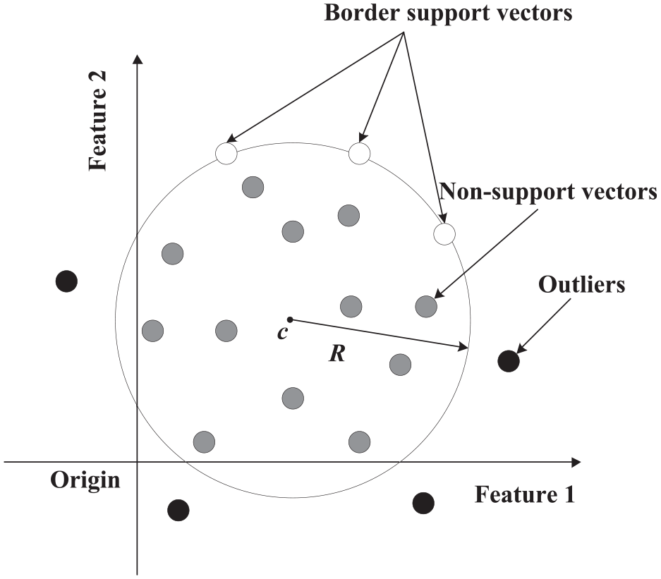
The QSSVM ¹⁶ first centers the dataset at the origin in their feature space before modeling a quarter sphere to encompass as many data points as possible. By doing this, it can convert the quadratic optimization problem of equation (2) to a linear optimization problem. The geometry of the QSSVM is displayed in Figure 3.

Figure 3.

Geometry of the hypersphere-based QSSVM.

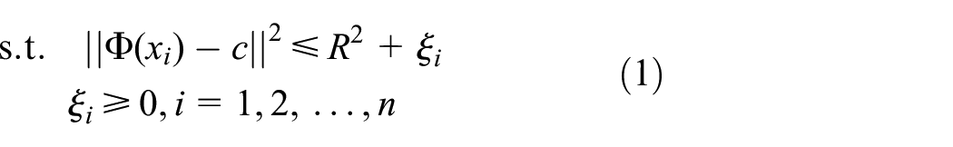
In Figure 3, R is the radius of the modeled quarter-sphere surface, which encompasses the majority of the data points in the feature space. Thus, the optimization problem of a QSSVM classifier is formalized as follows

$$\underset{R,\xi ,c}{min}{R}^2+\frac{1}{\nu n}\sum _{i=1}^n{\xi }_i$$

$$\begin{array}{c}\mathrm{s}.\mathrm{t}.||\mathrm{\Phi }(x_i)|{|}^2\le R^2+{\xi }_i\hfill \\ {\xi }_i\ge 0,i=1,2,\dots ,n\hfill \end{array}$$

(4)

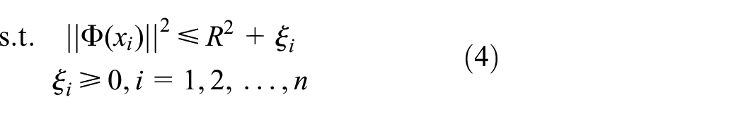
We also employ the Lagrange multiplier method to solve the formulation of equation (4). Then, the dual problem of equation (4) can be formulated as

$$\underset{\alpha }{min}-\sum _i{\alpha }_{i}k(x_i,x_i)$$

$$\begin{array}{c}\mathrm{s}.\mathrm{t}.\sum _i{\alpha }_i=1\hfill \\ 0\le {\alpha }_i\le \frac{1}{\nu n},i=1,2,\dots ,n\hfill \end{array}$$

(5)

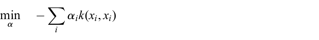
If a distance-based kernel is used when solving equation (5), such as the radial basis function (RBF) kernel, the inner products of the mapped data vectors (i.e. $k(x_i,x_i)$ ) are equal for all data vectors. Thus, there is no meaningful solution to equation (5). This problem can be solved by centering the kernel matrix of the feature space as follows ¹⁶

$$\mathrm{\Phi }\prime (x_i)=\mathrm{\Phi }(x_i)-\frac{1}{n}\sum _{i=1}^n\mathrm{\Phi }(x_i)$$

(6)

Then, the centered kernel matrix $k_c=〈{\mathrm{\Phi }}_c(x_i),{\mathrm{\Phi }}_c(x_i))〉$ can be obtained by

$$k_c=k-1_{n}k-k{1}_n+1_{n}k{1}_n$$

(7)

where $k=k(x_i,x_i)$ and $l_n$ is an $n\times n$ matrix with all values equal to $1/n$ .

After centering the kernel matrix in the feature space, the norms of the kernel are no longer equal and $k(x_i,x_i)$ of equation (5) can be replaced by the diagonal elements $k_c(x_i,x_i)$ of the kernel matrix $k_c$ .

After solving equation (5), data instances can be classified by their corresponding Lagrange multipliers: ${\alpha }_i=0$ implies that $x_i$ lies inside the quarter sphere, indicating it is a normal instance; ${\alpha }_i=1/\mathrm{vn}$ implies that $x_i$ is an outlier because it falls outside the quarter sphere; and $0<{\alpha }_i<(1/\mathrm{vn})$ implies that $x_i$ is a margin support vector.

Characteristics of data vectors reduced by DBN

The data collected by sensors is becoming increasingly high-dimensional, making outlier detection a challenge. We downloaded four real datasets from the UCI datasets. ²³ The four datasets include gas sensor array drift (GAS) with 128 dimensions, human activity recognition (HAR) using the smartphone with 561 dimensions, daily and sports activities (DSA) with 315 dimensions, and forest cover type (FCT) with 54 dimensions. We randomly mixed 5% stochastic anomalies with these four datasets (the detailed method is described in section “Datasets”) and compressed them by DBN. The compressed data vectors of the four datasets are plotted in Figure 4. For convenience, we only plot the distributions of two dimensions.

Figure 4.

Distributions of features extracted by DBN: (a) GAS, (b) HAR, (c) DSA, and (d) FCT.

After the dimensionality reduction, two phenomena emerge as follows:

1. Outliers are typically asymmetrically distributed, that is, all outliers in the four datasets are distributed on one side of the normal data. As the center of the sphere modeled by the OCSVM is calculated from all of the input data, the one-sided distributed outliers may lead to a biased center. However, the QSSVM fixes the center to the origin and maps the data to the quarter-sphere space. As the QSSVM considers the data instances that are close to the origin as normal, it performs effectively on the datasets with one-sided outliers.

2. After the dimensionality reduction by DBN, a clearer separation appears between the normal records and outliers, especially for the GAS and FCT datasets, which has also been demonstrated by Erfani et al. ¹⁵ As a result, the new method online QSSVM (OQSSVM) can be modeled in the input space after a dimensionality reduction of the data, to avoid the calculation of a highly complex kernel function in the feature space.

In summary, it is appropriate to model the QSSVM in the input space to perform outlier detection on the datasets that have been compressed by DBN. In the following sections, we will combine DBN with an online QSSVM model, which can accurately and efficiently detect large-scale and high-dimensional outliers in an online manner.

Fast outlier detection algorithm forhigh-dimensional sensor data

In this section, we first introduce an overview of our DBN-OQSSVM method. Then, we specifically introduce the OQSSVM model, including an efficient model training strategy to learn the optimal radius of the model and an online model testing strategy to detect outliers.

Method overview

Combining the functional characteristics of the DBN model and OQSSVM, we propose a new hybrid model DBN-OQSSVM for outlier detection. The DBN part consists of several RBMs, as indicated in Figure 5. The raw data are input into DBN, and the output of the DBN is used as an input for the OQSSVM. In the hybrid model, DBN is used as a dimensionality reduction tool to transform the data from high- to low-dimensional space, and OQSSVM is utilized as an outlier detection tool to identify outliers in large-scale datasets using a sorting method instead of solving an optimization problem.

Figure 5.

DBN-OQSSVM hybrid model.

There are two main advantages of using the DBN to preprocess the raw data: (1) the DBN can increase the disparity between the outliers and normal records ¹⁵ (also verified by our experimental results); and (2) the computational complexity can be significantly reduced when the dimensions of the input data are reduced.

The model training and testing processes are shown in Figure 6. For the training stage, we first use the training dataset to train the DBN model, and then we obtain the trained DBN model as well as the compressed vectors of the training set. We use the compressed vectors to train the OQSSVM model, and finally, we obtain the radius of the quarter sphere by a sorting method. For the testing stage, we first reduce the dimensions of the testing dataset using the trained DBN model, and then we identify the outliers through a decision function.

Figure 6.

Model training and testing for DBN-OQSSVM.

Online quarter-sphere one-class SVM

In this section, we introduce our OQSSVM method that can efficiently and accurately perform outlier detection after the dataset has been compressed by DBN. The OQSSVM model improves the original QSSVM model by much efficient model training as well as online model testing.

Efficient model training in input space

To reduce the computational time and space, we first introduce Theorem 1, ²⁴ and then propose Theorem 2 to efficiently obtain the radius of the quarter sphere.

We use $d_i$ to denote the kernel $k(x_i,x_i)$ in equation (5). For all input vectors, we first sort $d_i$ in descending order and obtain a sequence $\{d_{i\prime }|1\le i\prime \le n\}$ . By replacing $k(x_i,x_i)$ in equation (5) by $d_{i\prime }$ , the problem becomes

$$\underset{\alpha }{min}-\sum _i{\alpha }_i{d}_{i\prime }$$

$$\begin{array}{c}\mathrm{s}.\mathrm{t}.\sum _i{\alpha }_i=1\hfill \\ 0\le {\alpha }_i\le \frac{1}{\nu n},i=1,2,\dots ,n\hfill \end{array}$$

(8)

Theorem 1

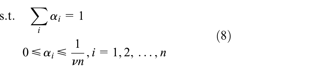
The square of the radius R for the quarter sphere obtained by solving equation (8) equals $d_{j\prime +1}$ , where $j\prime =\lfloor \nu n\rfloor$ . This is formulated by

$$R^2=d_{j\prime +1},j\prime =\lfloor \nu n\rfloor$$

(9)

Proof

Refer to the proof in the literature. ²⁴ □

As the DBN can separate most outliers from the normals in the input space, we model the quarter sphere in the input space, avoiding the computation of a large-scale kernel function. First, definitions for the model are provided and a theorem to rapidly train the model is then proposed.

Definitions

Let $\overline{x}=(1/n)\sum _{i=1}^n{x}_i$ , and ${\lambda }_i=(x_i-\overline{x})(x_i-\overline{x}{)}^T$ . We sort ${\lambda }_i(1\le i\le n)$ in descending order and obtain an ordered sequence $\{{\lambda }_{i\prime }|1\le i\prime \le n\}$ .

Theorem 2

For the training set $\{x_i|1\le i\le n\}$ , the square of the radius R for the OQSSVM in the input space equals ${\lambda }_{j\prime +1}$ , where $j\prime =\lfloor \nu n\rfloor$ . This is formulated by

$$R^2={\lambda }_{j\prime +1},j\prime =\lfloor \nu n\rfloor$$

(10)

Proof

As the OQSSVM fixes the center of the data on the origin, all training data will be centralized around the center, $\overline{x}$ , when the sphere is modeled in the input space. The optimization problem of the OQSSVM can be formalized as follows

$$\underset{R,\xi ,c}{min}{R}^2+\frac{1}{\nu n}\sum _{i=1}^n{\xi }_i$$

$$\begin{array}{c}\mathrm{s}.\mathrm{t}.||x_i-\overline{x}|{|}^2\le R^2+\xi \hfill \\ {\xi }_i\ge 0,i=1,2,\dots ,n\hfill \end{array}$$

(11)

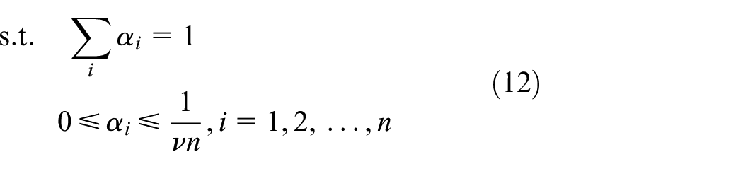
Thus, the dual problem for equation (11) can be formulated by

$$\underset{\alpha }{min}-\sum _i{\alpha }_i{\lambda }_i$$

$$\begin{array}{c}\mathrm{s}.\mathrm{t}.\sum _i{\alpha }_i=1\hfill \\ 0\le {\alpha }_i\le \frac{1}{\nu n},i=1,2,\dots ,n\hfill \end{array}$$

(12)

After sorting ${\lambda }_i$ in descending order, we have $R^2={\lambda }_{j\prime +1}$ and $j\prime =\lfloor \nu n\rfloor$ , according to Theorem 1. □

Based on Theorem 2, the training process for the DBN-OQSSVM can be dramatically simplified. The pseudo-code of the model training is presented in Algorithm 1. It inputs a historic dataset X of $n$ rows (instances), $d$ columns (dimensions), and a prior outlier rate $\nu$ ; it outputs the trained DBN model and radius R of the OQSSVM. Algorithm 1 first uses the training dataset X to learn the parameters in the DBN model, meanwhile obtaining the dimension-reduced dataset $\tilde{\mathbf{X}}$ (line 1). It then calculates the center of X and assigns $\lambda$ by the centered inner product (lines 2 and 3). Finally, it sorts the set of $\lambda$ in descending order and selects the $(\lfloor \nu n\rfloor +1)\mathrm{th}$ largest item as the radius of the OQSSVM (line 4).

Algorithm 1: Model training algorithm for DBN-OQSSVM in input space

Input: $\mathbf{X}=\{x_i,x_i\in \mathbb{R},i=1,2,\dots ,n\},$ $\nu$ Output: $R,M_{\mathrm{DBN}}$ 1 $[M_{\mathrm{DBN}},\tilde{\mathbf{X}}]\leftarrow \mathrm{trainDBN}(\mathbf{X})$ 2 $\overline{\mathbf{x}}\leftarrow \mathrm{mean}(\tilde{\mathbf{X}})$ 3 $\lambda \leftarrow (\tilde{\mathbf{X}}-\overline{\mathbf{x}})(\tilde{\mathbf{X}}-\overline{\mathbf{x}}{)}^T$ 4 $R\leftarrow \mathrm{sort}(\lambda ,\prime \mathrm{descending}\prime ,\lfloor \nu n\rfloor +1)$ 5 return $R,M_{\mathrm{DBN}}$

Online model testing

To efficiently perform the outlier detection in an online manner, a decision function is designed to determine whether the newly arriving data, $x$ , is an outlier. We first centralize $x$ in the input space by

$$x\prime =x-\overline{x}$$

(13)

and then determine the state of $x$ by the decision function as follows

$$f(x)=\mathrm{sgn}(R^2-x\prime x{\prime }^T)$$

(14)

where $R$ is the learned radius of the OQSSVM obtained by Algorithm 1. $x\prime x{\prime }^T$ is the inner product of $x\prime$ , representing the distance between $x\prime$ and the origin in the input space. If the inner product of $x\prime$ exceeds $R^2$ , the decision function will be assigned to $-1$ , and $x$ will be considered as an outlier.

Algorithm 2 presents the pseudo-code for the online detection algorithm DBN-OQSSVM. It inputs the new arriving data $x$ , learned DBN model, and learned radius $R$ ; it outputs the detecting result $y$ . Algorithm 2 first reduces the dimensions of $x$ using the learned DBN model (line 2) and centralizes $\tilde{x}$ (line 2). It then calculates the inner product $d\prime$ of the data vector $x\prime$ (line 3) and compares $d\prime$ with $R^2$ . If the inner product is greater than $R^2$ , $y$ is assigned to $-1$ (i.e. $x$ is an outlier) else $y$ is assigned to $1$ (i.e. $x$ is a normal instance) (lines 5–7).

Algorithm 2: Online model testing algorithm for DBN-OQSSVM
Input: $x$ , $M_{\mathrm{DBN}}$ , $R$ Output: $y$ 1 $\tilde{x}\leftarrow \mathrm{degradation}(M_{\mathrm{DBN}},x)$ 2 $\tilde{x}\prime \leftarrow \tilde{x}-\overline{x}$ 3 $d\prime \leftarrow \tilde{x}\prime \tilde{x}{\prime }^T$ 4 if $d\prime >R^2$ then5   $y\leftarrow -1$ 6 else7   $y\leftarrow 1$ 8 return $y$

The complete algorithm details

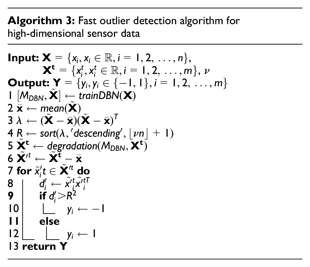
The pseudo-code of the complete outlier detection algorithm is presented in Algorithm 3. It inputs a training dataset $\mathbf{X}$ of $n$ rows (instances), $d$ columns (dimensions), a testing dataset ${\mathbf{X}}^{\mathbf{t}}$ of m rows (instances), $d$ columns (dimensions), and a prior outlier rate $\nu$ ; it outputs the detecting results of the testing data $\mathbf{Y}$ . Algorithm 3 first uses the training dataset $\mathbf{X}$ to learn the parameters in the DBN model and obtain the compressed training set $\tilde{\mathbf{X}}$ (line 1). It then calculates the center of the training set and assigns $\lambda$ by the centered inner product (lines 2 and 3). The radius of the OQSSVM is obtained by sorting $\lambda$ in descending order (line 4). To determine whether the data in ${\mathbf{X}}^{\mathbf{t}}$ are normal or abnormal, Algorithm 3 first reduces the dimensions of ${\mathbf{X}}^{\mathbf{t}}$ using the learned DBN model (line 5) and centralizes the compressed data into ${\tilde{\mathbf{X}}\prime }^t$ (line 6). For each data point in ${\tilde{\mathbf{X}}\prime }^t$ , it calculates the inner product $d{\prime }_i$ of the data vector (line 8) and compares $d{\prime }_i$ with $R^2$ . If the inner product is greater than $R^2$ , $y_i$ is assigned to $-1$ (i.e. $x_i^t$ is an outlier) else $y_i$ is assigned to $1$ (i.e. $x_i^t$ is a normal instance) (lines 10–12).

Algorithm 3: Fast outlier detection algorithm for high-dimensional sensor data

Input: $\mathbf{X}=\{x_i,x_i\in \mathbb{R},i=1,2,\dots ,n\}$ , ${\mathbf{X}}^{\mathbf{t}}=\{x_i^t,x_i^t\in \mathbb{R},i=1,2,\dots ,m\}$ , $\nu$ Output: $\mathbf{Y}=\{y_i,y_i\in \{-1,1\},i=1,2,\dots ,m\}$ 1 $[M_{\mathrm{DBN}},\tilde{\mathbf{X}}]\leftarrow \mathrm{trainDBN}(\mathbf{X})$ 2 $\overline{\mathbf{x}}\leftarrow \mathrm{mean}(\tilde{\mathbf{X}})$ 3 $\lambda \leftarrow (\tilde{\mathbf{X}}-\overline{\mathbf{x}})(\tilde{\mathbf{X}}-\overline{\mathbf{x}}{)}^T$ 4 $R\leftarrow \mathrm{sort}(\lambda ,\prime \mathrm{descending}\prime ,\lfloor \nu n\rfloor +1)$ 5 ${\tilde{\mathbf{X}}}^{\mathbf{t}}\leftarrow \mathrm{degradation}(M_{\mathrm{DBN}},{\mathbf{X}}^{\mathbf{t}})$ 6 ${\widetilde{\mathbf{X}\prime }}^t\leftarrow {\tilde{\mathbf{X}}}^{\mathbf{t}}-\overline{\mathbf{x}}$ 7 for $\tilde{x}{\prime }_i^t\in \tilde{\mathbf{X}}{\prime }^t$ do8   $d{\prime }_i\leftarrow {\widetilde{x\prime }}_i^t{\widetilde{x\prime }}_i^{\mathrm{tT}}$ 9  if $d{\prime }_i>R^2$ 10    $y_i\leftarrow -1$ 11  else12    $y_i\leftarrow 1$ 13 return $\mathbf{Y}$

Evaluation

In this section, we compare the performance of our method DBN-OQSSVM with DBN-OCSVM, ¹⁵ DBN-QSSVM, and iForest ¹⁸ through extensive experiments.

Competitors

DBN-OCSVM

DBN-OCSVM ¹⁵ first compresses the raw data by DBN and then models the surface of a minimum hypersphere which can encompass as many instances as possible in the feature space. Instances outside the border are identified as outliers.

DBN-QSSVM

DBN-QSSVM first compresses the raw data by DBN as well. Then, the compressed data are centered at the origin in their feature space. Finally, the surface of a minimum quarter hypersphere is modeled, which can encompass the majority of the centered instances.

IForest

iForest ¹⁸ is an isolation-based outlier detection method. It randomly partitions all instances recursively to generate a binary tree. Outliers are expected to be isolated closer to the root. As the isolation does not require any distance or density measures, it avoids the optimization problem with high computational complexity. However, since each partition is randomly generated, individual trees are generated with different sets of partitions. It generally needs to generate abundant trees to converge the path lengths of each instance.

Datasets

In our experiments, We used four different types of real datasets from the UCI Machine Learning Repository ²³ to verify the performance of the four methods, including a GAS with 128 dimensions, HAR using smartphones with 561 dimensions, DSA with 315 dimensions, and FCT with 54 dimensions. The GAS dataset is collected by 16 chemical sensors, each of which records 8 features, including steady-state feature, the exponential moving average, and transformation of feature sets. The data records in HAR are obtained from accelerometer and gyroscope three-axial raw signals. For each signal, the HAR database records its characteristics such as the mean value, standard deviation, signal magnitude area, and signal entropy. The DSA dataset records the motion sensor data of 19 DSA, including sitting, standing, lying on the back and on the right side, ascending and descending stairs, and standing in an elevator still. The FCT dataset records the environmental features of forests, including elevation, aspect, slope, and horizontal. For all of the datasets, we selected 5000–50,000 consecutive records; 80% for the training data and the remaining 20% for the testing data.

By referring to the experimental settings in Erfani et al., ¹⁵ we normalized all datasets in the range [0,1], and then randomly select 5% and 10% records in training and testing sets, respectively. For each selected record, we replaced it with a random value drawn from the uniform distribution function U(0,1) to simulate an outlier.

Metrics

The four methods are evaluated using two metrics:

1. Area under the curve (AUC): AUC is the area under the receiver operating characteristic (ROC) curve, indicating the overall accuracy of a classification method.

2. Computational time: the training time is the period starting from an algorithm inputting the training dataset and the necessary parameters until the trained model is output. The testing time is the period starting from an algorithm inputting the testing dataset until the testing results are output. QSSVM is an offline method whose training and testing processes can only be implemented simultaneously. We only record the overall time of QSSVM. Because algorithms for DBN-OCSVM, DBN-QSSVM, and DBN-OQSSVM cost the same amount of time on the DBN training and testing, we only record the time required for the SVM training and testing.

Model settings

When comparing the three methods of DBN-OQSSVM, DBN-QSSVM, and DBN-OCSVM, the structure of DBN (including the number of epochs, units on the hidden layers, and learning rate) was set based on the best performance of the three methods. ²⁵ For the FCT and GAS datasets, the OCSVM and QSSVM have a similar accuracy under the linear kernel and RBF kernel. As the linear kernel is much more efficient compared to the RBF, ²⁴ we apply a linear kernel to the OCSVM and QSSVM for the FCT and GAS datasets. However, for HAR and DSA, the accuracy of OCSVM and QSSVM can be notably improved by RBF kernel. Therefore, we use RBF kernel in the OCSVM and QSSVM on HAR and DSA. Because the predefined outlier ratio, $\nu$ , influences the accuracies of the three methods to different degrees, we also vary $\nu$ in our experiments to evaluate their performances.

For the iForest method, we set the subsample size to 256 and the number of trees to 100 based on its best performance in terms of efficiency and accuracy. The results presented in the following sections were averaged over 100 executions. All methods were implemented with MATLAB 2017a, running on a server with a quad-core CPU at 1.90 GHz and 32GB RAM.

Results

Overall performance

Table 1 displays the AUC, training, and testing times for the four methods on different datasets. In the table, $\nu$ is set to 0.05, 0.08, and 0.15 for the OQSSVM, QSSVM, and OCSVM, respectively, based on their best performance. The number after “DBN” represents the number of hidden layers in the DBN structure (e.g. DBN1 has one hidden layer, DBN2 has two hidden layers, and DBN3 has three hidden layers). The following conclusions can be made from Table 1: (1) the improved outlier detection method DBN-OQSSVM provides an averaged AUC greater than 99%, which is about 3% higher than DBN-QSSVM, 5% higher than DBN-OCSVM, and 5% higher than iForest; (2) on average, the training and testing time of OQSSVM are only 0.14% and 0.35% of DBN-OCSVM, respectively, and 0.93% and 0.43% of iForest, respectively, which demonstrates that the new method is much more efficient than the competitors; and (3) the structure of the DBN does not seem to influence the accuracies of the three methods significantly but slightly affects the DBN training and testing times. Deeper DBN requires slightly more time for model training and testing. More experiments on different DBN structures are provided in the following section.

Table 1.

Overall performance results.

DBN structure	SVM method	Metric	Datasets (dimensions)				Avg.
			GAS (128)	HAR (561)	DSA (315)	FCT (54)
		DBN training time (s)	0.2310	0.3871	0.3126	0.1954	0.3102
		DBN testing time (s)	0.0021	0.0030	0.0025	0.0019	0.0025
DBN1		AUC	0.9891	0.9989	0.9933	0.9998	0.9938
	OQSSVM	SVM training time (s)	0.0007	0.0007	0.0007	0.0007	0.0007
		SVM testing time (s)	0.0002	0.0002	0.0002	0.0002	0.0002
		AUC	0.9564	0.9597	0.9578	0.9573	0.9578
	QSSVM	SVM time (s)	0.1669	0.2229	0.2222	0.1622	0.1936
		AUC	0.9369	0.9411	0.9483	0.9387	0.9421
	OCSVM	SVM training time (s)	0.2552	0.7860	0.7895	0.2114	0.5105
		SVM testing time (s)	0.0290	0.0895	0.0862	0.0242	0.0572
		DBN training time (s)	0.2384	0.3929	0.3200	0.2012	0.3171
		DBN testing time (s)	0.0021	0.0030	0.0025	0.0019	0.0026
DBN2		AUC	0.9907	0.9999	0.9950	0.9998	0.9952
	OQSSVM	SVM training time (s)	0.0006	0.0007	0.0008	0.0007	0.0007
		SVM testing time (s)	0.0002	0.0002	0.0002	0.0002	0.0002
		AUC	0.9574	0.9597	0.9578	0.9573	0.9581
	OQSSVM	SVM time (s)	0.1678	0.2264	0.2232	0.1627	0.1950
		AUC	0.9440	0.9429	0.9499	0.9483	0.9452
	OCSVM	SVM training time (s)	0.2552	0.7981	0.8011	0.2116	0.5165
		SVM testing time (s)	0.0287	0.0901	0.0921	0.0243	0.0588
		DBN training time (s)	0.2430	0.3988	0.3247	0.2052	0.3222
		DBN testing time (s)	0.0021	0.0030	0.0026	0.0020	0.0027
DBN3		AUC	0.9912	0.9999	0.9953	0.9999	0.9955
	OQSSVM	SVM training time (s)	0.0006	0.0007	0.0008	0.0007	0.0007
		SVM testing time (s)	0.0002	0.0002	0.0003	0.0002	0.0002
		AUC	0.9573	0.9597	0.9578	0.9571	0.9580
	QSSVM	SVM time (s)	0.1681	0.2271	0.2232	0.1633	0.1954
		AUC	0.9442	0.9429	0.9501	0.9483	0.9457
	OCSVM	SVM training time (s)	0.2566	0.8040	0.8000	0.2111	0.5179
		SVM testing time (s)	0.0285	0.0896	0.0910	0.0240	0.0583
		AUC	0.9349	0.9449	0.9553	0.9519	0.9468
	iForest	iForest training time (s)	0.0671	0.1030	0.0686	0.0608	0.0749
		iForest testing time (s)	0.0421	0.0640	0.0374	0.0421	0.0464

DBN: deep belief network; SVM: support vector machine; GAS: gas sensor array drift; HAR: human activity recognition; DSA: daily and sports activities; FCT: forest cover type; AUC: area under the curve; QSSVM: quarter-sphere SVM; OCSVM: one-class support vector machine.

The bold values highlight the comparison on method accuracy.

Sensitivity test on DBN structure

To verify the performance of our method under different DBN structures, we vary the number of hidden-layer units as well as the output-layer units (i.e. the dimension for the compressed data) in our experiments. The hidden layer varies from 20 to 38 and the output layer varies from 2 to 10. From Figure 7, the structure of DBN seems not to influence the accuracy of our method much. More specifically, as the number of hidden-layer units changes, the change in the AUC is no more than 0.32%; as the number of output-layer units changes, the change in the AUC is no more than 0.46%.

Figure 7.

AUC for DBN-OQSSVM over different DBN structures: (a) GAS, (b) HAR, (c) DSA, and (d) FCT.

Sensitivity test on $\nu$

The AUCs of the three algorithms under different $\nu$ are plotted in Figure 8. $\nu$ represents the estimation of the outlier rate in the training set. From Figure 8, as $\nu$ increases, all curves in the figures increase first and then tend to decrease after reaching their peaks. The DBN-OQSSVM always provides a better AUC than those of the DBN-QSSVM and DBN-OCSVM. On average, the DBN-OQSSVM can improve the AUC by approximately 11%. The optimal value of $\nu$ for the DBN-OQSSVM just equals the ratio of the outliers we set in our experiments, while the optimal value for DBN-OCSVM is greater than the ratio. This also indicates that as affected by one-side distributed outliers, the DBN-OCSVM requires a relatively larger $\nu$ than the actual outlier ratio.

Figure 8.

AUC for three algorithms over different $\nu$ : (a) GAS, (b) HAR, (c) DSA, and (d) FCT.

Scalability test

Figure 9 compares the overall computing time (averaged over the four datasets) of the four methods on different scales of datasets. From the figure, the time of the DBN-OQSSVM is considerably less than those of the DBN-OCSVM, DBN-QSSVM, and iForest by up to three orders of magnitude. Even for the dataset with 50,000 records, DBN-OQSSVM only requires less than 10⁻³ second to output the outliers, while DBN-OCSVM and DBN-QSSVM require close to 10 s and iForest requires about 3 s. This is because, during the training phase, the radius of the OQSSVM is obtained by sorting, whereas both the OCSVM and QSSVM compute the radius by solving an optimization problem. In the testing phase, the decision function of equation (14) in our method only requires the inner product, whereas the decision function of equation (3) in DBN-OCSVM method requires the computation of the high-dimensional kernels. iForest needs to construct 100 binary trees to obtain the average length of paths for each instance. The testing data needs to traverse each of the trees as well to obtain its average height. The results in Figure 9 also demonstrate that compared to the competitors, our method is more appropriate for large-scale datasets.

Figure 9.

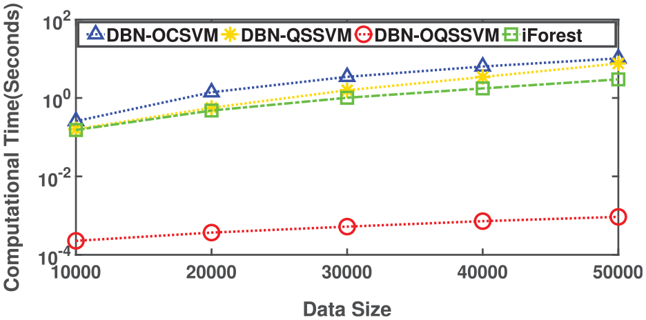
Computational time of the four methods under different dataset scales.

Conclusion

In this article, we proposed a fast outlier detection method DBN-OQSSVM for high-dimensional and large-scale data collected by WSNs. The method DBN-OQSSVM first reduces the dimension of the observations by the DBN. It then fixes the center of the datasets to the origin in the input space and calculates the radius of the quarter sphere using a sorting method. Finally, based on the learned radius, outlier detection is performed in an online fashion. We compared our method with three competitors through extensive experiments on four real WSN datasets. The experimental results strongly confirm the satisfactory performance of our method.