Method for rapid deployment of low-cost sensors for a nationwide project in the Internet of things era: Air quality monitoring in Taiwan

Abstract

When the air quality problem of PM_2.5 first raised public attention and an emerging low-cost sensor technology appeared suitable as a monitoring measure for said problem, Taiwan’s Environmental Protection Administration devised a nationwide project involving large-scale sensor deployment for effective pollution monitoring and management. However, the conventional siting optimization methods were inadequate for deploying thousands of sensors. Therefore, this study develops a rapid deployment method. The current results may serve as a reference for the Taiwan government for use in the aforementioned nationwide project, which is an environmental Internet of things–based plan involving 10,200 sensors to be deployed throughout the country. The four monitoring targets are classified as types of industry, traffic areas, communities, and remoteness, and a three-phase implementation structure is devised in the method. The open-source geographic information system software named QGIS was used to implement the proposed method with relevant spatial data from local open-data resources, which generated new, necessary geographic features and estimated sensor deployment quantity in Taiwan. The deployment result of the 10,200 sensors is 4790 in the type of industry, 708 of the traffic area, 3935 of the communities, and 767 of remoteness. The proposed method could serve as a useful foundation for the sensor deployment of environmental Internet of things. Policymakers may apply this method to budget allocation or integrate this method alongside conventional siting methods for the modification of deployment results based on the local monitoring requirements.

Introduction

Air pollution is a very significant environmental and social issue. At the same time, it is a complex problem posing multiple challenges in terms of management and mitigation of harmful pollutants.^1,2 Particle matter is one of the Taiwan’s most problematic pollutants in terms of health. During 2018, all designated national air quality automatic continuous monitoring stations measured particulate matter (PM₁₀ and PM_2.5) and annual mean concentrations along with standard deviation at 42.9 and 19.0 μg/m³, while the corresponding standard deviation was 11.4 and 5.1 μg/m³. ³

X Zhou et al. proposed low-cost and portable sensor technology which appeared suitable as a monitoring measure for the aforementioned issue. The sensors are available to measure PM_2.5, CO, CO₂, and volatile organic compounds (VOCs) with the features of technical feasibility, light weight, and low power consumption. The technical feasibility of low-cost sensor depends on multiple criteria including accuracy, precision, response and recovery time, zero-drift, resolution, and sensitivity. ⁴ Use of low-cost air quality sensor networks has been deployed mainly according to subjective judgment or systematic strategy suggested by experts, with main sites including airports, chemical clusters, and urban areas.^5,6

While citizens nowadays value the importance of air quality much more, Taiwan’s Environmental Protection Administration (EPA) advocates the intellectual concept of “Development and application of the environment Internet of things (IoT) sensor network” ⁷ in order to promote environmental governance and the quality of public service. The ultimate goal is to make the environment IoT sensor network an important part of the smart city, to strengthen our ability to monitor air quality, and also to apply the newly developed information technology—IoT. Through the deployment of low-cost sensors to monitor the air quality in streets minute-by-minute, SC Chang et al. presented that the IoT can support and intensify the application of existing national monitoring sites that the EPA uses to provide air quality information, making the data more precise and clear. ⁸

The deployment of air sensors was considered an air quality monitoring network (AQMN) siting problem in the past. The assumption behind the AQMN problem was that the regulatory monitoring stations were expensive, and the objective of the AQMN siting was often cost minimization or restriction. Before beginning a deployment network assessment, the purposes of the network had to be reviewed and prioritized. SM Raffuse et al. introduced networks that were likely to be used to meet a variety of purposes, such as monitoring compliance with the U.S. National Ambient Air Quality Standard (NAAQS), public reporting of the air quality index (AQI), assessment of population exposure to pollutants, assessment of pollutant transport, monitoring of specific emissions sources, monitoring of background conditions, evaluating models, and possibly others. Site-by-site analyses, bottom-up analysis, and network optimization techniques were used in different environmental scenarios. ⁹

The studies of conventional siting have consequently used optimization methods. S Gage et al. ¹⁰ proposed environmental applications which typically employed spatial data derived from visually apparent mediums for the area of interest. We thus devised the rapid deployment method as a policy tool to assist decision-makers and stakeholders to obtain a comprehensive view of low-cost sensor monitoring.

The rapid deployment method

Based on the spatial manipulation, the rapid deployment method is devised as three phases (Figure 1): the preparation phase, the implementation phase, and the modification phase. In the preparation phase, the steps include the objectives setting, elimination rules, and the spatial data preparation. The implementation phase explores the deployment of the aforementioned steps in the preparation phases, including unnecessary area elimination, deployment density determination, and regular point algorithm execution. In the modification phase, one can redefine the deployment density and the results for further discussion.

Figure 1.

The structure of the rapid deployment method.

The algorithm is based on the estimated number of sensors, and the resulting deployment positions can subsequently be used as reference for actual deployment. Factors which must be taken into account in actual deployment of sensors include shelter, power supply, online transmission, and geographic environment before looking for proper deployment sites in the neighborhood of reference positions. While sensors are capable of detecting air-pollution density within a radius of 500–1000 m, the higher the deployment density, the easier it is to capture features of local pollution and spatial changes.

Deciding monitoring targets

The first step of the rapid deployment method is to determine the management scope by setting the targets. We can decide on the targets by asking the questions which concern us most, such as how the possible polluting sources act, how the communities near industrial areas are influenced, as well as identifying whether there are any accidental pollution issues happening in remote areas. Figure 2 lists the four monitoring targets, including the industrial areas (industry), high traffic areas (traffic), communities near industrial areas (community), and remote areas (remoteness). For each type of industry, the purpose is to track the pollution source. For the type of traffic, the purpose is to monitor the pollution level in the near environment. For the type of community, the sensors are supposed to monitor pollution for nearby residents to protect their health. For the type of remoteness, the sensors are deployed to enhance the monitoring coverage to detect accidental pollution in the areas of low population density.

Figure 2.

The four targets.

The study was meant to meet the actual needs of Taiwan. The problems were defined after discussion with officials of Environmental Protection Administration in Taiwan and the study resorted mainly to the tracing of pollution sources and monitoring of public health. It covered fixed pollution sources, such as discharges by industrial zones, and mobile pollution sources, such as automobile and motorcycle exhaust. Due to Taiwan’s limited space and high population density, pollution of communities by neighboring industrial zones occurs frequently, and pollution resulting from open burning in the remoteness still causes health issues.

Deciding elimination rules

Eliminating unnecessary areas is an essential step for conventional siting to save on computation resources and to assist policymakers in focusing attention on essential areas. Subsequently, elimination rules should be decided in the method for following process. Some elimination rules identify unsuitable heights for sensor deployment and existing sensors that were previously installed.

Spatializing the targets

The aforementioned objectives need to be spatialized for deployment computation. For example, if we set the target to monitor a type of industry, we need spatial data of all industrial areas to plan sensor deployment around these areas for the implementation phases. Once we set a target, relevant spatialized data need to be found or generated. In other words, this step prepares the base deployment map of several layers for the following spatial manipulation. Each layer of the map is prepared for each target, which means that each raw spatial data is processed for each objective as a layer for the base map. For example, when we choose two objectives of industrial monitoring and community protection, the county layer is required to be cropped out of the industrial area as a new layer for the base map. If one cannot find or generate the relevant spatial layer, one should consider modifying the target until the relevant spatial layer can be generated.

Eliminating unnecessary areas

This is the first step in the implementation phase. Prior elimination of unnecessary areas is essential, because it can increase decision clarity in advance by ruling out those areas that should not be included. Based on the given elimination rules, one needs to transform the rule into a spatial manipulation step to alter the deployment base map.

Defining the deployment density

Before the next step, deployment density needs to be determined. Since the regular point algorithm is the main step for the deployment method, the essential subsequent step is to set the deployment density. The deployment density represents the importance of each target. Instead of using weight in the conventional optimization method for siting, higher deployment density can be used to emphasize the relevant objective.

Executing the regular point algorithm

After the aforementioned steps have been determined, this main step yields the final results. The principle of the algorithm is to generate regular points in a specific polygon given the relevant attributes, mainly the density or the distance between any two points. From a spatial analysis view, the processed map is made up of several layers of numerous polygons, each with different attributes.

Another geo-algorithm can be used here for the auxiliary purpose of count points in the polygon, which will generate a new attribute of the number of the points in each polygon after the implementation of the regular point algorithm. For each goal, summarizing the new attribute will obtain the final results for the deployment quantity for each objective.

Redefining the deployment density

Although the results will be generated by the previous steps, decision-makers will probably not be satisfied with the results when they try to adjust the density settings to compare different cases.

Inversing the results to the square of the density

According to the new deployment density, as long as the same base map is being used, it is possible to obtain a modified result by quick estimation from the square ratio. This step will be demonstrated in the following sections.

The limitations of the proposed methodology

The method employed geographic information system (GIS) as the main tool. In case of insufficient data, users can consider using other spatial data in monitoring. For instance, due to the inability to secure real-time emission data of factories flues in Taiwan, the study employed industrial-zone coverage as a substitute.

As for the number of sensors, users can adjust deployment density or targets to gradually meet restrictive conditions by referring to the practice of the modification phase.

With GIS as the main tool, the study divided, according to the four targets, spatial data into polygons without mutual interference, such as traffic locations focusing on urban areas with high population density, and communities addressing residential areas in the neighborhoods of industrial zones. Therefore, the four deployment scenarios and conditions in this article are defined as independent incidents, without any overlapping and supplementing among them. Each deployment site may meet the demands of two or more scenarios.

Software and open-data sources

The spatial analysis software used herein is QGIS 2.18.27 (QGIS Development Team, 2019). QGIS is responsible for overlaying the spatial data to generate new geographic features, that is, new polygons, to present the aforementioned monitoring targets. Afterward, two geo-algorithms are used to further implement the deployment method, defined as the “regular point algorithm” and the “count points in the polygon.” These are built-in functions in QGIS. The regular point algorithm is used for generating the points with regular distance, and the “count points in the polygon” algorithm is used to sum up the points that are located in different scenarios for the monitoring targets. The relevant spatial data are from the open data archives in Taiwan (data.gov.tw, 2019). Here are the lists of the relevant data used in this article.

1. Boundaries of Taiwan, including all cities and boroughs: https://data.gov.tw/dataset/7442

2. Boundaries of the industrial areas in Taiwan: https://data.gov.tw/dataset/25598

3. Population statistics spatial data: https://data.gov.tw/dataset/25128

4. Road networks: https://data.gov.tw/dataset/73232

5. Digital terrain model data: https://data.gov.tw/dataset/35430

For demonstration of the implementation phase, the main part in the method, we make a package of the required data and a QGIS processing model and uploaded it at the link: http://tinyurl.com/rapid-deployment-model, including a “0ReadMe.doc” file for instruction. One could understand the practical steps from this model and could modify it to apply for the cases for similar goals.

Case study

In this study, we have used Taiwan as the example for the deployment issue. Taiwan is mountainous, with an average population density of about 640 people per km². There are 180 industrial areas in Taiwan, most of them located in the western plains of the island.

In the national plan, 10,200 sensors were deployed. We started applying the method to estimate the number of different deployment distribution scenarios, which are described in next sections.

Deployment may be subject to the constraints of land acquisition and power supply, as well as consideration of safety and deployment altitude. Via simulation, this article proposed 10,200 deployment sites as a reference for local telecom carriers which must conduct on-site inspection to select sites with lampposts, signal posts, and telecom boxes for deployment.

Deciding monitoring targets

The targets selected were industrial monitoring, traffic monitoring, community monitoring, and remoteness monitoring.

Deciding elimination rules

The elimination rule considered here was for height. Since Taiwan is a mountainous island, and maintenance is difficult if installed in the high areas, the rule was set to a maximum of 500 m. Any area higher than 500 m was ruled out in the deployment process.

Spatializing the targets

Once we decided on the targets based on the type of industry, traffic, community, and remoteness, as shown in Figure 3, we needed to spatialize these objectives to implement the deployment process. Each objective was converted into a spatial layer. For industrial area monitoring, the industrial area distribution map was the main map for the following deployment. For community monitoring, we used the population density map as the main map, since we primarily focused on the people who were possibly influenced by industrial pollution. For remoteness, population density was also used to identify low population density areas. For traffic monitoring, the road network can be found. To identify the high traffic roads, we overlaid the road network and the population map to crop the relevant roads with a high population density area. Afterward, we buffered the cropped roads with 250 m as our main layer for the following process.

Figure 3.

The processed base map.

Eliminating unnecessary areas

Following the eliminating rule (see section “Deciding elimination rules”), we removed the areas above 500 m using digital terrain model data, and the manipulation process, as shown in Figure 4.

Figure 4.

Map generation showing application of elimination rules.

Defining the deployment density

After determining the targets, we emphasized their importance by defining the deployment density for each target. For each type of industry and traffic, we set 300 m as the deployment density, meaning that we set each sensor at 300 m. As for each type of community and remoteness, we set sensors at 1500 and 5000 m, respectively. The deployment density setting is illustrated in Figure 5.

Figure 5.

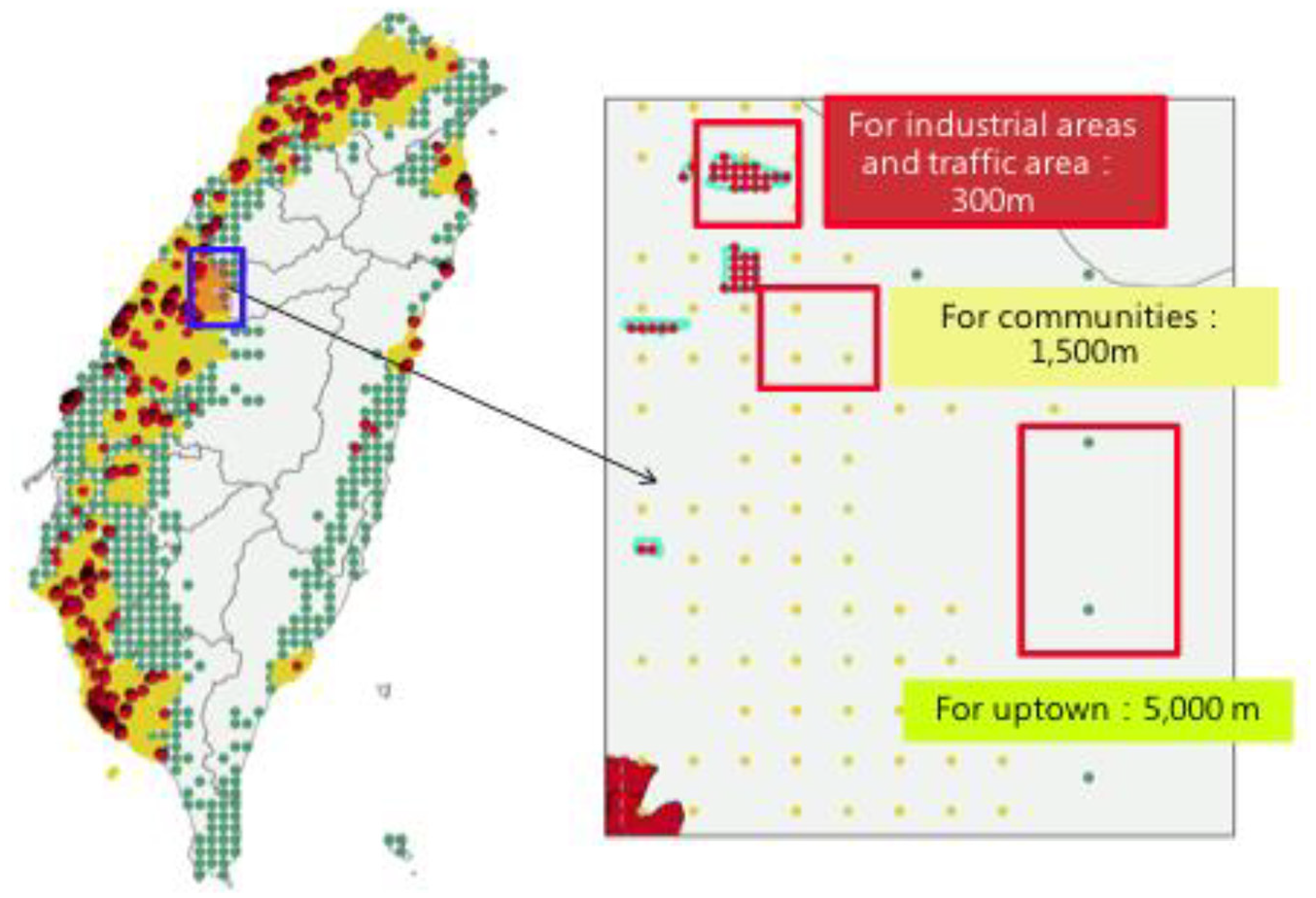
The deployment density determination.

Executing the regular point algorithm

According to the above rules, the calculation was implemented mainly by the regular point algorithm. The result for each type of industry was 4790 points, as illustrated in Figure 6, and was 708 points for each type of traffic, as illustrated in Figure 7. For each type of community, the result was 3935 points, as illustrated in Figure 8, and for each type of remoteness, it was 767 points, as illustrated in Figure 9. The number of points for industrial monitoring was the largest, and the number for traffic areas was the smallest. If the cost for each deployment is the same, the ratio for each type represents the budget allocation.

Figure 6.

The result of the type of industry.

Figure 7.

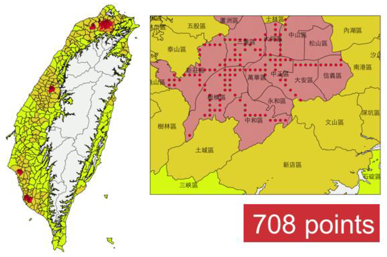
The result of the traffic areas.

Figure 8.

The result of the communities.

Figure 9.

The result of remoteness.

Redefining the deployment density

Decision-makers may alter the results generated by the algorithm by redefining the deployment density to discover other possible alternating results. For example, if decision-makers would like to see the results emphasizing the type of industry rather than other targets, they can modify the deployment density, for example, by modifying 300–600 m.

Inversing the results to the square of the density

Once the decision-makers have defined a new density according to the feature of the algorithm, the number of results can be adjusted by the inversion of the square of the new density. For example, if the density setting changes from 300 to 600 m, the number will be a quarter of the original results. This step allows stakeholders who have their own interests to reach a consensus. Moreover, this step’s nonlinearity allows users to estimate the results by intuition, such that the alternating estimation continues until the stakeholders can reach agreement. Finally, when the limit of the number of sensors is fixed, such as 10,200 mentioned in the national plan in Taiwan, the density modification can also be used to meet the requirements of the plan.

Nevertheless, the method still focuses on deployment of fixed sensors to meet demands of the Environmental Protection Administration for tracing pollution sources, which needs continuous monitoring of numerical values. For mobile sensors, refer to the number of fixed model deployments.

Conclusion

The proposed rapid deployment method could serve as a useful foundation for the sensor deployment of environmental IoT. Policymakers may find it beneficial to integrate this method alongside conventional siting methods for the modification of deployment results based on the local monitoring requirements. Also, we believe that the method could overcome the disadvantages of conventional methods and assist policymakers in prioritizing and allocating resources in a fast-paced, policy-making context. In discussion around our national plan, we found that the sensor deployment also assisted us in allocating the budget and defining local government responsibility.

In the first three steps of the preparation phase, the monitoring targets and reasonable deployment density can be defined based on one’s experience. However, it is difficult to reach the final results due to multiple concerning factors and the nonlinearity of deployment.

In the implementation phase, one can observe the power of integrating the open data. The GIS tool can rapidly generate the deployment results without tedious field investigation and complicated optimization. For the rapid development of technology, we find that this rapidity is required and necessary in the decision-making process and the national plan discussion.

In the modification phase, the final results can be altered for preferred sensor deployment density to observe the changes accordingly. These changes will be helpful when stakeholders have to seek consensus. Moreover, the GIS also provides spatial observations that can help stakeholders visualize changes in possible locations for those sensors that are within the regions of their concern, even though the locations may be hypothetical.

This methodology can be extended in other applications. Since one can implement the conventional siting methodology, such as optimization model implementation, based on the number of suggested deployments by this method for a specific region. This rapid method has not been developed to provide a complete solution, but to provide a rapid estimation that can allocate resources such as budget and devices when the decision process is time critical.