
Abstract
In copper mining, there are two main separation processes: leaching for oxidized minerals and flotation for sulfide minerals. In Chile, the increase of sulfide minerals in the deposits and the decrease of oxidized minerals have led to an increase in the investigation of flotation processes and the optimization of their associated operations. One of the concentration processes is the use of thickeners, whose main objective is to treat the tailings that leave the plants in pulp form with approximately 30% solids and obtain a pulp with a concentration greater than 50% with clear water flow. The recovery of water is the main goal, so knowing the concentration profiles of solids and sedimentation is crucial. However, the characteristics of the pulp and the operation of the thickeners are complex because a great variety of forms can be found in the concentration profile of said pulp. This limits conventional measurement techniques and makes it difficult to apply deterministic models to the solids profile, given the high nonlinearities and variability of the system. In this article, a solution is proposed by developing a sensor that allows the online estimation of sludge level and concentration of solids, based on a model of neural networks (with the model of Maxwell for dispersions), allowing to measure the solids profile regardless of the operating conditions. The structure selected has nine inputs with a hidden layer, two neurons, and two outputs being trained with tailings from Chuquicamata, obtaining the information from a 50 L pilot with 10-electrode bar of 60 cm of length, resulting in an estimation error of 0.8 cm with a network of 26 parameters.
Introduction
The processing of sulfide minerals incorporates in its process a solid-liquid separation stage called thickening. Thickeners are widely used in the early stages of the tailings generation process. This is the process by which solids and liquids are separated by gravity through the phenomenon of sedimentation and consolidation in cylindrical tanks called thickeners. The performance of this process depends on the settling velocity of the solid particles, the latter can be increased by the agglomeration of particles, usually through the addition of flocculants. In addition, thickeners are equipped with a rake mechanism that helps move the “underflow” sediment. 1
These are essential clarifiers that produce a current of “overflow” clear water. Design considerations are based on the sedimentation gradient of the slowest particle and minimum disturbance conditions of the mean water current where the solid particles settle. 2 Gravity thickeners provide a treatment of vast volumes of diluted sludge that are transported to the tailings pond, with the intention of dissipating the kinetic energy from the incoming streams and discharging from this current into the main volume of the pond. 3
The current methodology that allows calculating operational parameters such as calibration that is based on the electrical consumption of the equipment, has silting problems, and prevents the dosing of reagents. Therefore, the variability of the sedimentation conditions generates solid profiles with diffuse interfaces and types of sedimentation highly dependent on the consumption of reagents. The dosage of reagents and mineralogy affects the degree of adherence of the particles and currently, there is no instrumentation that simultaneously measures the sludge level and the solids content. The problem of controlling this type of equipment arises, where it is important to accurately describe both the steady and dynamic state characteristics of the processes throughout the range of operation, including their nonlinear behavior. The first reason is that the mineral is exceptionally complex as a system compared to other materials such as those processed in the chemical industry, such as cellulose cement. The ore contains other minerals mixed with random variations in its properties (grain size, content, association, micro-fractures, and distribution of characteristics on the surface). A second reason is that the physics and chemistry of the sub-processes involved are not understood in their entirety. 4 This limits conventional measurement techniques and makes it difficult to apply deterministic models to the solids profile, given the high nonlinearities and variability of the system as proven by other investigations.5–7
Due to this last problem, an appropriate methodology for the characteristics of the process is studied, focusing on the use of artificial intelligence. Artificial intelligence techniques are becoming one of the most used due to their simple implementation, easy design, robustness, and flexibility. They have been widely used in the field of chemical engineering, for modeling, process control, and classification, including several branches such as artificial neural networks, fuzzy logic, genetic algorithms, expert systems, and hybrid systems. 8 This can be found, for example, in the simulation of a semi-industrial thickener plant based on computational fluid dynamics to investigate the effects of the thickener on the parameters’ performance. 3 In recent years, the mining industry in Chile has begun to use and observe an increase in interest in artificial intelligence techniques in processes such as the estimation of copper production, where traditional methods tend to lack certainty and knowledge. One of these techniques is softcomputing. 9 On-line monitoring reduces faults and optimizes production, as is also reflected in the implementation of an expert system in the crushing process of the Gabriela Mistral division, presenting an improvement of 2.17% and a decrease in detentions by 55%. 10 Another example is found in a combination of different types of simulators: dynamic processes, static metallurgy, distributed processes, control techniques, and strategies for complex processes. 11 Otherwise, in neural network applications, they can be successful in nickel high-pressure leaching, to reduce operational costs and increase the estimation accuracy of the model. 12
For this reason, a sensor based on the technology developed by Tavera et al. 13 is designed and improved based on intelligent electronic conductivity profiles with neural networks for online conductivity reading, with the incorporation of an estimative model of sludge height (interface height) and solid concentration. Basing it on neural networks allows to measure the solids profile with greater precision and accuracy, given the nonlinearity capabilities of the model. 14
Artificial neural networks are intelligent artificial systems capable of solving a range of complex problems. An artificial neural network is a computer system made up of units known as neurons. Neurons are interconnected processors that work in parallel to perform a given task. A training algorithm is used to adjust parameters such as weights and biases. 15 The minimum processing elements of neural networks are called artificial neurons and they are generally simplified as nodes. The performance of the neurons is assumed as a mapping of the junctions. In some cases, they can be considered as threshold units that fire when total input exceeds a certain bias level. Neurons usually operate in parallel and are configured in regular architectures. They are usually organized in layers and feedback connections with other layers are allowed. The strength of each connection is expressed by a numerical value called weight, which cannot be modified. The artificial systems of neurons work with the parallel distribution of computation of the networks, with its most basic characteristic being the architecture. Only some of their networks provide instant answers. Other networks take time to respond and are characterized by their domain behavior, which usually refers to their dynamics. Neural networks also differ from each other in their modes of learning. There are a variety of learning rules that establish when and how the weights of the connections change. 16 The category of reinforcement learning (RL) helps the system or agent learn from the experiences obtained in the environment through interactions and observing the results of these interactions. The interaction helps to imitate the basic patterns in which humans and animals learn. 17
A prototype instrument was developed to determine the sludge level and solids content in thickeners, applying a model of neural networks, designing and assembling a sensor with robust electronics for online monitoring of axial conductivity profiles in a 50-L pilot thickener, based on artificial neural networks for the estimation of sludge height and solid content in experimental form.
Electrical conductivity is the property of a substance to conduct electric current. It is defined by its symbol k.
Conductivity is the constant of proportionality in Ohm’s law

where i is the current density (A/cm2), Δv is the potential gradient (V/cm), and k is the conductivity (Ω−1 cm−1).
In the case of mineral pulps, the conductivity of the solution is in a range of 5000–15,000 μS/cm. When adding solids, the conductivity can vary by 1000 μS/cm.
The resistance of an electrolytic solution cannot be measured using direct current, because it changes the concentration of the electrolyte. The accumulation of electrolysis product of the electrodes also alters the resistance of the solution. Alternating current is used to overcome the effect.
The resistance of the electrolyte in parallel plates is given by equations (2) and (3)

where vA and vB are the potentials on the electrode plates and I is the current in the electrical circuit

where K is the conductance of the electrolyte. From equation (3) the term Acell/L refers to the cell constant (cc), expressed in centimeter (cm).
The conductivity measurement depends on the geometry of the electrode and the measuring range of the instrument. The conductivities method is a technique that is used to measure the volumetric content of dispersion, for example, pulp solids, organic drops in solution, gas in pulps or in solutions. In the case of pulps, the conductivity of the liquid–solid dispersion depends mainly on the conductivity of the solution and the volumetric content of the solid.
The Maxwell model considers a liquid (or continuous) phase that contains small spheres (solid or dispersed phase) of different conductivities. The effective conductivity of the dispersion kn is given by equations (4) and (5)

where kl is the conductivity of the liquid, and εd is the volume fraction of the solid content of the dispersion. Equation (4) can also be expressed as

To illustrate the sensitivity of the maxwell model, Figure 1 shows a graph of the volumetric fraction of the pulp and the variation of conductivity, depending on the percentage of solids, for a pulp finding in copper mining (dry solid density of 2.6 g/cm3 and solution conductivity of 10 mS/cm).

Volumetric fraction of the pulp and the variation of conductivity, depending on the percentage of solids.
Materials and methodology
Materials and system components
The multielectrode used to measure the conductivities was submerged inside the thickener and had holes for taking data at different heights; this allowed the maintenance or replacement of the electrodes in contact with the pulp (Figure 2).
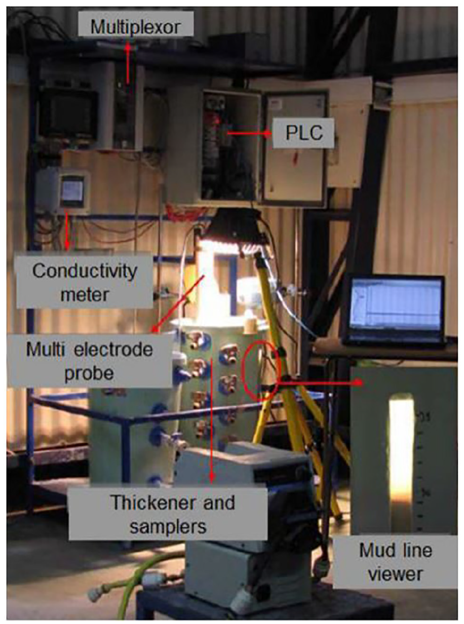
System used for the measurement.
Regarding the multielectrode bar, this consists of a cylinder made of high-density polyethylene (HDPE) and sealed at the top and bottom, as shown in Figure 3. Through a hole that crosses a part of the cylinder, a metal base (stainless steel) is fitted with thread inside. The electrode that captures the conductivity signal is also mounted on the metal base and, through wiring, the signal is sent to the programmable logic controller (PLC).

Multielectrode bar.
It is important to note that the geometry of the electrodes is linked to a cc, which in reality is affected by the geometry of the electrodes, varying with the environment to which it is exposed, as well as being exposed to faults such as wear and incrustation, caused by the abrasive environment. For this particular investigation, the geometry used for the electrodes was a disk, prioritizing the area increase, easy replacement of electrodes, and the cc. Three disks of 10, 20, and 30 mm diameters spaced from center to center at 5 cm are evaluated.
To establish the diameters of a theoretical flow area, a reduction of the electric field of 5% was considered after performing a simulation in the software electric field, version 2.01. The diameters were 2.8, 3.9, and 4.7 cm. For the disks, we have 10, 20, and 30 mm, respectively. However, to obtain the constants of real cells, it is required to calibrate the electrode bar with a solution with standard conductivities. Regarding the latter, the smallest deviation and without statistical bias corresponds to the 20 mm electrode.
Another point to evaluate in the geometry of the electrode is its inclination, a flat disk was chosen, because it does not present significant differences with a disk with an inclination of 15°. A diagram of the system is shown in Figure 4:
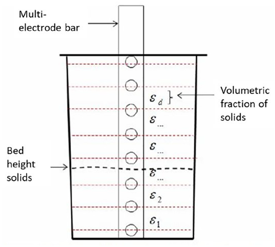
Diagram of the system.
The system components are listed as follows:
- PLC;
- Conductivity meter, Yokogawa (Mod. EXAxt450);
- Multiplexer, 10 electromechanical relays (RC-HF41-24VDC);
- Multielectrode bar, submersible probe whose electrodes mounted along with the bar measure conductivity at different heights of the medium where it is submerged;
- Tank systems (pilot thickener), two tanks that are connected by two peristaltic pumps for handling pulp. The pilot thickener is fed with pulp in the central part of the tank and its discharges are in the upper part with clear liquid and in the lower part with decanted solid. By regulation of flows in peristaltic pumps, the system allows varying the sludge height and the percentage of solids.
On-line capture of conductivity profiles requires programmable electronic components and also software logical components, which are necessary to perform data capture, historization, and subsequent information processing. For a better system understanding, data acquisition will be addressed explaining the hardware connectivity, separately of the logic needed to obtain online conductivity profiles for storage based on data (SQL Server 2005).
The hardware is composed of the PLC with the built-in rack of modules, a conductivity meter, and a multiplexer. The PLC has the function of sending a signal to an electromechanical relay to close or open the circuit in the conductivity measurement. In turn, the electromagnetic relays fulfill the function of multiplexing the signal since, through the opening and closing of the circuit, they are responsible for directing the conductivity signal at different heights of the pilot tank. Finally, the conductivity reading is taken by the conductivity sensor and its signal changes position according to the sequence programmed in the PLC.
Following the data flow, the human–machine interface (HMI) of Opto_22 receives and orders the signals captured by the instrument (status signal and conductivity); these signals are collected by an Opto_DataLink interface, which is responsible for sending the information to a database where finally the conductivity profiles captured by the instrumentation are stored. The use of MATLAB is included for data processing, generating models such as artificial neural networks.
The reading of signals delivered by the instrumentation must be read by an HMI, in the case of the PLC, the software used is the Pac Basic Control. The result of the programming of the storage procedure for the historization and acquisition of data in real time provides reliable information that is available for use once it has been processed and stored in the database.
Calibration of multielectrode sensor
The calibration processing is basically to obtain the value of the cc since, considering the way in which the electrodes are arranged and their type of geometry (disk-type electrodes), it is difficult to obtain the value based on their dimensions.
The procedure for calibrating the multielectrode bar is carried out by immersing the multielectrode bar in a liquid medium, maintaining a resistance measurement with the conductivity meter, in parallel with a portable conductivity meter, with a standard solution. Amounts of salt are added to the solution in order to vary the conductivity of the liquid medium.
The cc is also a function of the solution’s conductivity and that is because the field lines get closer together when the solution’s conductivity increases. The variation of conductivity in the solution in a mining plant is gradual in time, due to the effect of the accumulation of salts or seasonal effects. In the case of the Maxwell model, this effect is compensated, since the ratio of conductivities is used.
Neural network design
One of the problems of thickeners arises out of the characteristics of the solid (particle size, solid density, adhesion between particles) and variability of the process; the axial profile of solids concentration in the thickener takes various forms that are not represented by linear models.
A neural network model for determining variables such as sludge height and solids content can be tackled as a problem of approximating functions and as such, it can be approached using a model based on neural networks.
In particular, the use of conductivity profile measurements to estimate interfaces using neural networks has proved to be feasible, for example, in the detection of the foam interface in industrial flotation column. 18
The learning mechanism is the mechanism by which all the parameters of the network adapt and are modified. In the case of the multilayer perceptron, it is a supervised learning algorithm. The learning of the multilayer perceptron is equivalent to finding a minimum of the error function. 19
To keep the error function to a minimum, the presence of nonlinear activation functions is required.20,21 This makes the network response to be nonlinear with respect to the adjustable parameters, making the problem of error minimization a nonlinear issue, and as a consequence, nonlinear optimization techniques have to be used for resolution. One technique corresponds to backpropagation, in which the weights of the network move along the negative gradient of the error function. The backpropagation term is used due to the way of implementing the gradient method in the multilayer perceptron, as the mistake made in network output is propagated backward, transforming it into an error for each of the hidden neurons in the network. Downward gradient backpropagation algorithms are often too slow in practical problems, being a disadvantage while implementing a model in real time.
The fast training algorithm belongs to two categories. The first category uses heuristic techniques, which were developed from an analysis of the performance of the descending gradient algorithm. The second category of fast algorithms uses numerical optimization techniques.
For the numerical optimization category, in the MATLAB Neural Network Toolbox Tool, the performance of the following algorithms is evaluated:
- Levenberg–Marquardt;
- BFGS quasi-Newton;
- Resilient backpropagation;
- Scaled conjugate gradient;
- Conjugate gradient with Powell/Beale restarts;
- Fletcher–Powell conjugate gradient;
- Polak–Ribière conjugate gradient;
- One-step secant;
- Variables learning rate backpropagation.
For this evaluation, six different problems are used; three of them correspond to the recognition of patterns and the others correspond to problems of approximation of functions. Simulated data of these problems are constructed and the other four use real data.
For the problems of approximation of functions, the Levenberg–Marquardt algorithm and the scaled conjugate gradient algorithm have the fastest convergence. The Levenberg–Marquardt algorithm obtains a lower error than that of other algorithms tested.
There are many algorithms used to improve the generalization of a neural network model of which early detention and the automatic regularization have the best generalization process. The algorithms mentioned in improving the generalization of network meet the same goal but in the way they work, they are totally different.
As an example, when training a neural network with a small set of data, Bayesian regularization provides a better generalization than the early detention and this is because the Bayesian regularization does not require a data set (from the initial set) for the model validation.
Seven cases are analyzed in order to select the best generalization algorithm, all of different sizes and different numbers of fields in both the input layer and the output layer, where the mean square error is evaluated for the different data sets.
Bayesian regularization delivers better performance than early stopping. One of the disadvantages of the Bayesian regularization method is focused on the time of convergence, which is generally greater than in early stopping. In this way, it is concluded that the most appropriate structures are conjugate gradient with early stopping and Levenberg–Marquardt combined with automatic Bayesian regularization.
It is required to establish the number of hidden layers of the proposed network structures. For this, it is necessary to experimentally determine the least number of neurons in the hidden layer to minimize the adjustment error to that of established value.
Design of the tests for sensor validation
It was considered that in the case of sedimentation, it is possible to find at least four types of sedimentation, which indicate the sludge height and the concentration of solids.
The electrode bar of the prototype sensor is 60 cm long, the design of the proposed experiment is to use intervals of 5 cm; thus, for 10 electrodes spaced at 5 cm, nine levels of sludge height are obtained. If the four forms of sedimentation are used for a single solids content, 180 experiments (4 × 45) are required. Given the complexity that this implies, it is proposed as a strategy to train the neural network structures with simulated profiles and in this way determine the most appropriate number of layers, to subsequently validate experimentally.
For the calculation of conductivity, it is necessary to know the volume fraction of solids (εd) at different heights of the tank. Equations involved in obtaining the conductivities profile are presented as follows

where α corresponds to the type of solid, εdmin and εdmax are the minimum and maximum solid fraction within the tank, respectively. β is represented by different equations depending on the height of the sludge level and the measurement height. For measurement height greater than or equal to the height of the sludge level, β is given by the expression

For electrode height lower than the height of the sludge level, β is given by the expression

where α corresponds to the type of solid, Hmudlevel is the height of the sludge level, Hmeasurement is the height of the measurement, and Htank is the total height of the thickener, in our case of the pilot tank.
A database for the nine possible conductivity profiles with nine levels of sludge is generated. We have to determine the maximum number of neurons that can be used in the hidden layer since there is a limitation that is a function of the number of experiments of the data set for training the network.
Calculation of the number of experiments is required for a certain number of neurons in the hidden layer (a neuron in the output layer is considered)

where n is the number of neurons in the input layer, h is the number of neurons in the hidden layer, and s is the number of neurons in the output layer.
- Input layer: Nine neurons in the input layer, which are given by the number of measurements (nine measurements) in the conductivities profile delivered by the hardware.
- Hidden layer: The hidden layer is where three structures that correspond to 2, 3, and 4 are to be evaluated.
- Output layer: The number of neurons in the output layer is given by the deliverable, that is, the solids content and sludge height of the tank (two neurons).
Each neural network structure is trained separately with four data sets corresponding to flocculent settling (set 1), semi-flocculent settling (set 2), semi-discrete settling (set 3), and discrete settling (set 4), as shown in Figure 5.
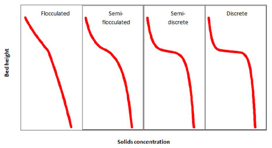
Possible forms of sedimentation.
Each training takes randomly 70% of the data set for training, 15% for internal validation, and 15% to evaluate the model. Random cross-validation was used. The training is repeated five times, to test the robustness of the program. The evaluation of the different algorithms and neural network structures are carried out in MATLAB software. The model with the best fit is that of Levenberg–Marquardt with three neurons in the hidden layer, this for sludge height and for the percentage of solids in the tank.
Generalized model fit for all types of curves
Levenberg–Marquardt with three neurons presents the least number of errors, making it the best option to be used combined with the automatic Bayesian regularization for the generalized model.
As a methodology, a database for all cases of sedimentation will be used, and 3, 5, 9, and 11 neurons will be evaluated in the hidden layer, since in this case 176 profiles have been simulated. This strategy will allow to visualize if an increase in neural networks improves the estimation.
For the optimization of neural networks, 70% of the data is used to train, 15% for internal validation, and 15% of the data to evaluate the model, the latter are independent and have not been used in network optimization. Sampling for training, validation, and evaluation is done randomly and 30 repetitions are carried out to evaluate this sampling.
The results for a scan of 2–11 neurons in the inner layer with 30 repetitions each is shown in Figure 6, which presents the error average adjustment of the data used to evaluate (15% of the sample), and their respective measurements.
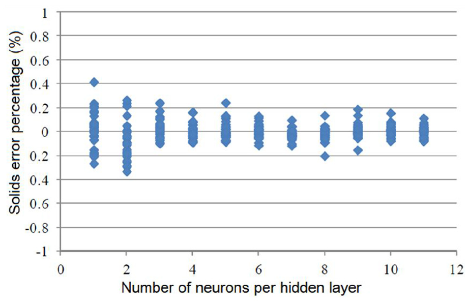
Solids error percentage.
Results and discussion
Results for solids percentage
Results for a scan of 2–11 neurons in the inner layer with 30 repetitions each are shown in Figure 6, which presents the error adjustment average of the data used to evaluate (15% of the sample), and their respective measurements. To visualize the degree of dispersion of the data, the standard deviations of fit are also presented in Figure 7.

Error standard deviation.
In Figures 8–10, the regression graphs are presented for the cases of three, five, and nine neurons, with two repetitions each.
Regression graphs for three neurons (two replicates).

Regression graphs for five neurons (two replicates).

Regression graphs for nine neurons (two replicates).
The error associated with the percentage of solids varies between ±0.2% of solid, as shown in Figure 6. In addition, the standard deviation of the solids percentage error (Figure 7) shows a decrease when working with three neurons in the hidden layer, deviations that remain constant for larger hidden layers. The aforementioned, added to the correlation coefficients greater than 0.999 (Figures 8–10), allows concluding that the optimal number of neurons in the hidden layer for fitting the percentage of solids is three neurons.
Results for sludge height
For the sludge height, it can be seen that the error of the model is between ±0.8 cm (Figure 11).

Sludge height error.
The standard deviations graph of sludge height error (Figure 12) shows a downward trend as the number of neurons in the hidden layer increases, a deviation that increases when the seven neurons are exceeded. To visualize the degree of dispersion of the data, the standard deviations of fit are also presented in Figure 12.

Error standard deviation for sludge height.
Given that the variation of the standard deviations does not present major differences, and that the correlation coefficients are greater than 0.99, it is concluded that for fitting the sludge height, the optimal size of the hidden layer is between two and three neurons. In Figures 13–15, the regression graphs are presented for the cases of three, five, and nine neurons, with two repetitions each.

Regression graphs for three neurons (two replicates).

Regression graphs for five neurons (two replicates).
Regression graphs for nine neurons (two replicates).
Experimental validation with tailings
As an experimental result, a total of 71 profiles are obtained and two of them are shown in Figure 16. Two inflection points are observed, the upper one corresponding to the sludge line or clearwater pulp interface and the second inflection corresponding to the line of compaction or consolidation of solids.
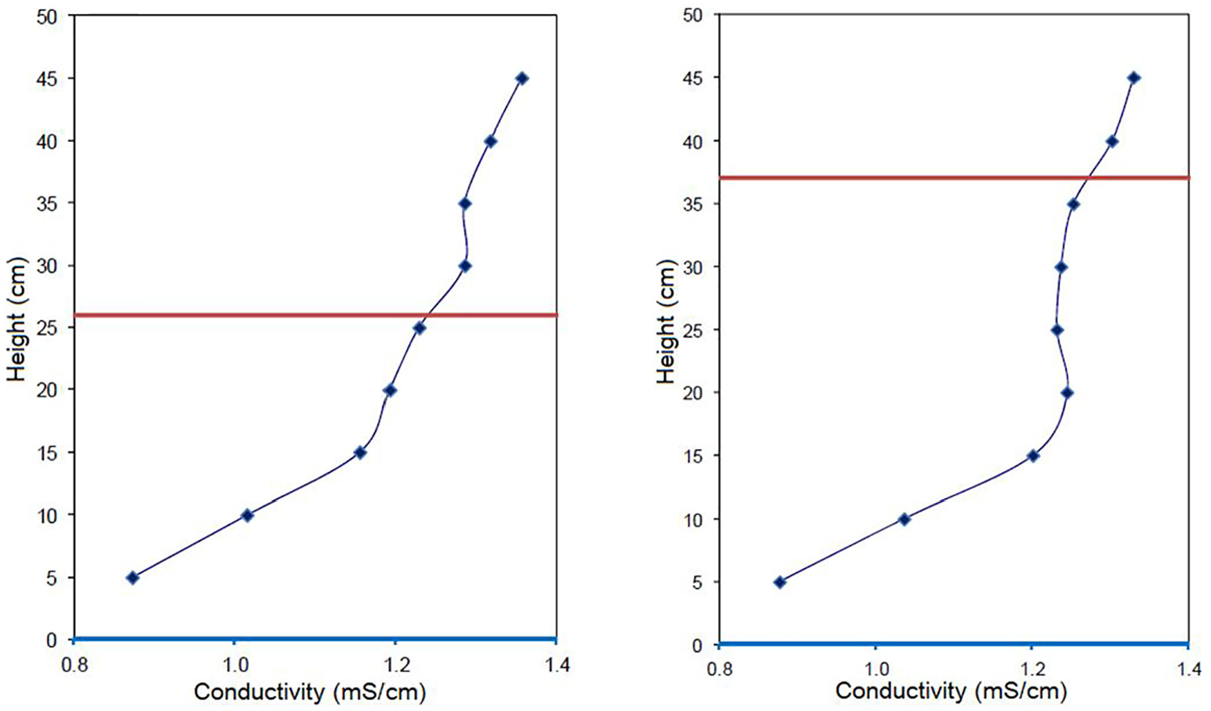
Examples of conductivity profiles obtained experimentally.
From these profiles and the selected network architecture, the calibrations of the neural network are carried out, in order to reduce the error in the estimation and to minimize the number of parameters required.
Validation and calibration of the neural network with three neurons with a hidden layer
The network structure with one hidden layer and three neurons is calibrated, with sigmoidal transfer function. Since the number of experimental data is 71 points (total of conductivity profiles) and to minimize the amount of training data, 60% of the data is used for adjustment or calibration (55% training and 5% internal validation) and 40% of the experimental data for independent validation. In this case, 39 set data are used for a network structure with 38 parameters. Since the data for training and the data for testing are randomly selected in the adjustment of the neural network parameters, it is necessary to repeat the training processes to obtain the statistical significance of the adjustment and to calculate the adjustment errors. In this case, 30 workouts or repetitions are performed, where the average adjustment error is plotted for each of the repetitions (Figure 17). In addition, and to establish the level of error dispersion, the standard deviation is plotted as shown in Figure 18.
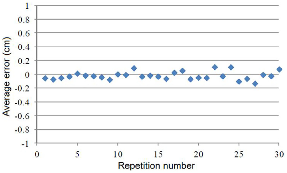
Average error for each repetition—three neurons with a hidden layer.

Adjustment error standard deviation for each repetition—three neurons with a hidden layer.
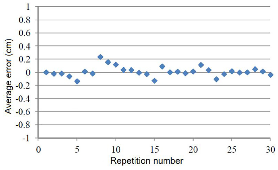
From Figures 17 and 18, it is concluded that it is possible to adjust the height of sludge with neural networks from conductivity profiles in a consistent way. In addition, adjustment errors are maintained, with a maximum dispersion of 0.8 cm (twice the maximum standard deviation).
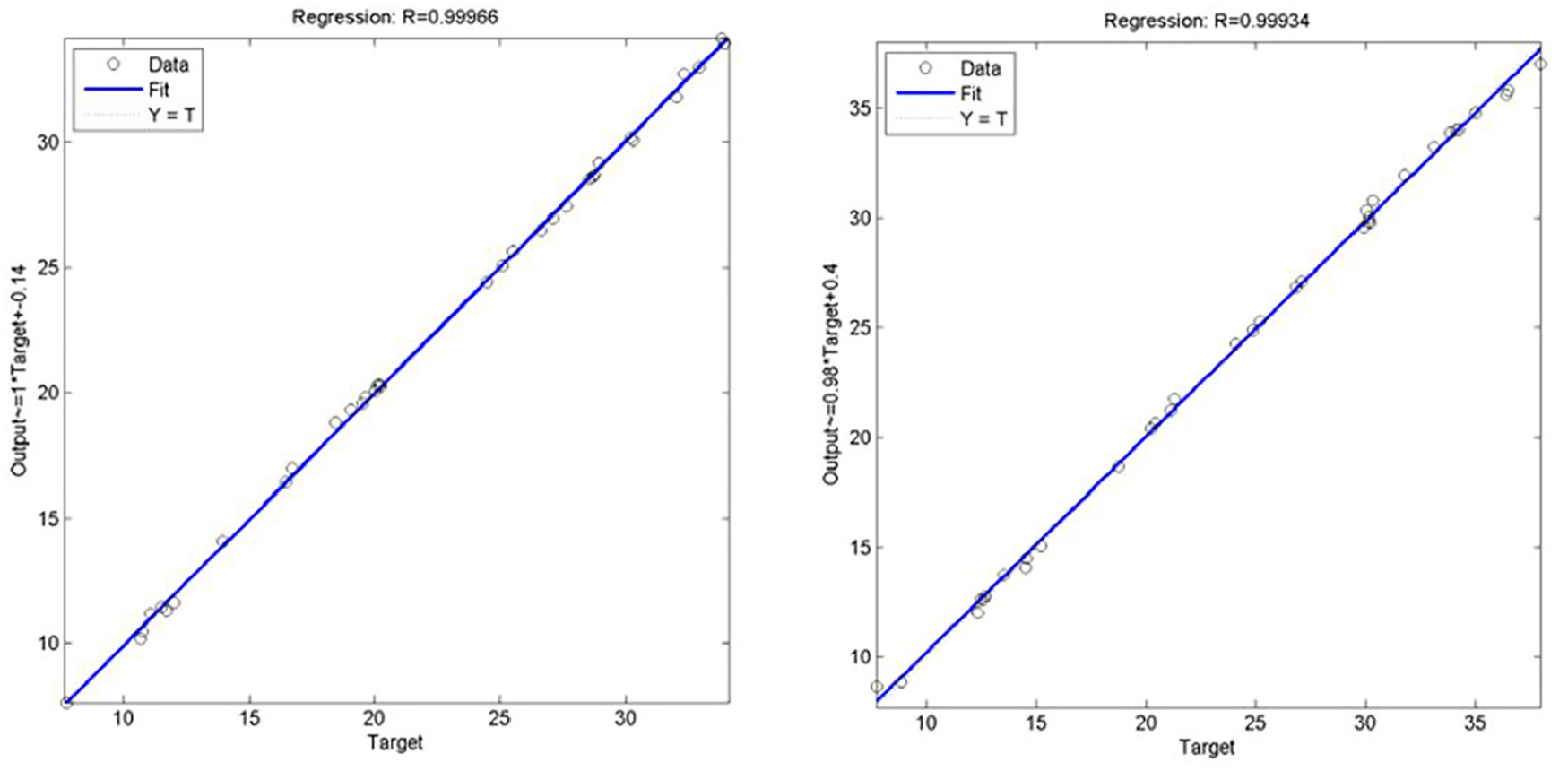
As a result of this adjustment, the regression between experimental data and the estimation of the neural model is presented. In this case, three hidden layers (Figure 19), for 100% of the data (includes training 55%, internal validation 5% and 40% validation with data independent of network optimization). From Figure 19 (replicates 14 and 19), a high level of correlation is observed (over 0.999) and a low bias (under 0.03 cm). A grouping of data is also observed for low interface levels (under 28 cm of mud), this due to the fact that due to the operating condition, the compaction of mud at that height is achieved more quickly. Notwithstanding the foregoing, the experimental data cover the entire range of the pilot equipment (25–45 cm).
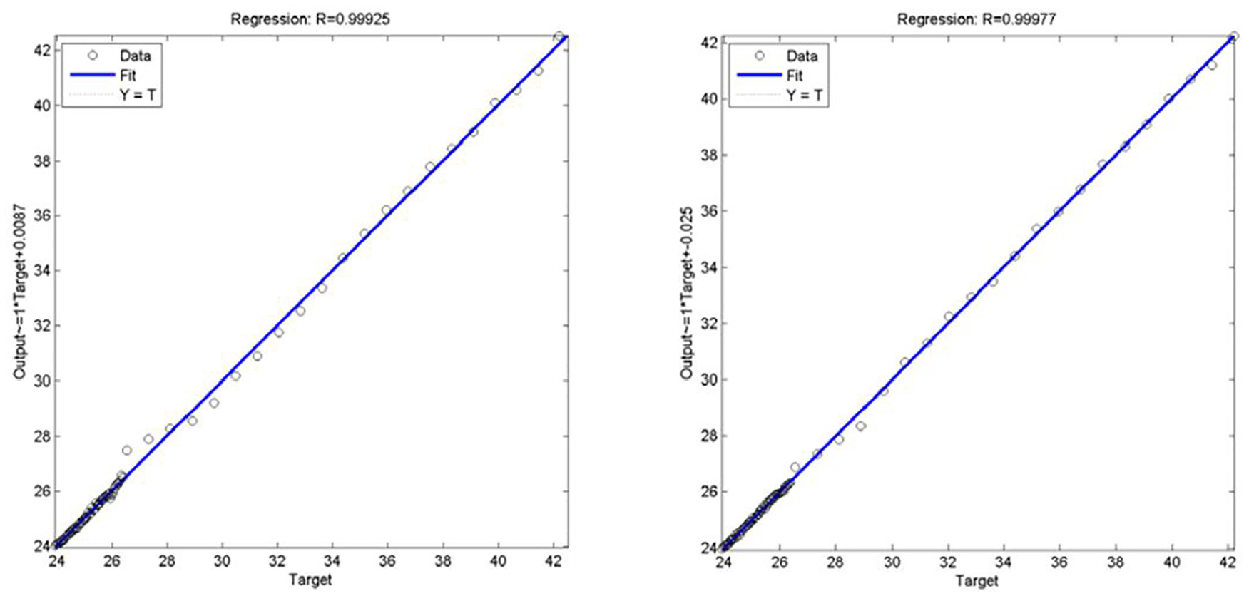
Regression for three neurons in hidden layer (repetitions 19 and 14), for 100% of the data.
In the case of validation, 40% of the remaining data is used, and the results of the adjustment are presented in Figure 20.

Regression for three neurons in hidden layer (repetitions 1 and 2), for the data used in validation (40%).
From Figure 20, a high degree of correlation is also observed between the fitted model and the experimental data. In addition, random data sampling maintains the entire range of the experiment (25–45 cm of sludge), a condition that is maintained for all replications.
For the case of this experiment with 71 experimental data and a network with nine inputs, two outputs, and three neurons in the hidden layer, 38 parameters are required, which requires a greater number of training data, and in this case, validation data are restricted to 40%. Considering the network structure, for the case of the level, it presents low errors for two and three neurons (Figure 12).
Validation and calibration of the neural network with three neurons with a hidden layer
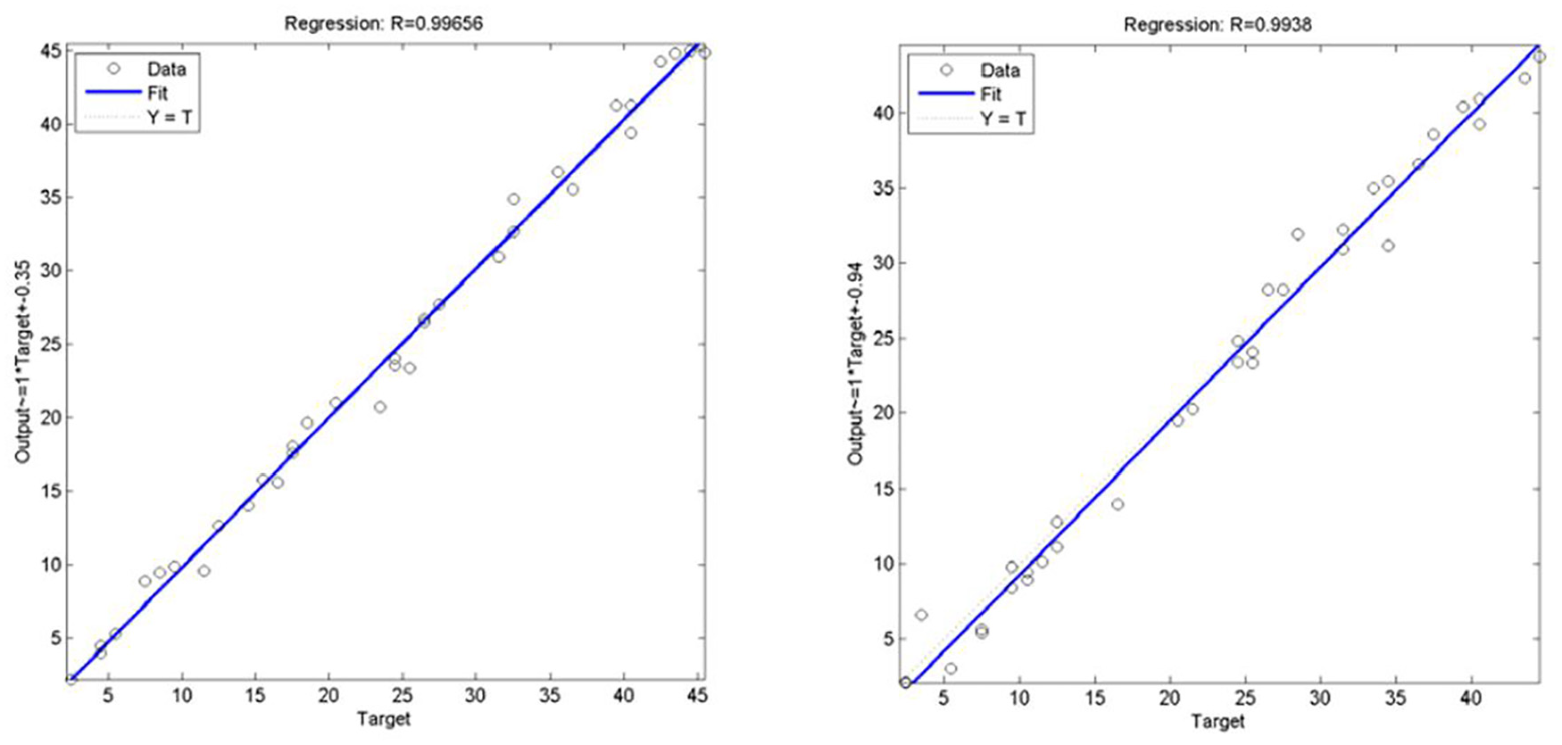
When using a 9 × 2 × 2 architecture, 26 parameters are required, and therefore, the number of experimental data is reduced to 27, with this the percentage of data that can be used in the validation reaches 57%, which gives greater validity to the model; however, the cost is to reduce the accuracy of the fit.
When analyzing the results of the fit for 30 repetitions, it is observed that the average errors (Figure 21) are in a ±0.2 cm range, just like in the three neurons case, with only one case above this range; therefore, there are no significant differences in the average adjustment error.
Average error for each repetition—two neurons with a hidden layer.
In the same way, when graphing the standard deviation of the fit for each repetition (Figure 22), a specific case is observed over 0.6 and in general deviations of the order 0.2 to 0.3 cm. As a consequence, no significant deviations are observed when using two neurons, which is consistent with the simulated data analysis that compares the standard deviation of the fit with the number of neurons in the hidden layer (Figure 12).

Adjustment error standard deviation for each repetition—three neurons with a hidden layer.
The adjustment results for the validation case (57% of the data) are presented in Figure 23.
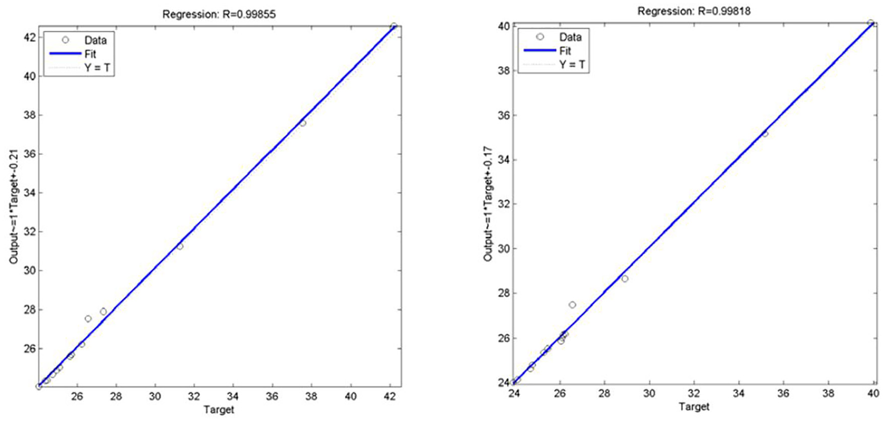
Validation of the model with two neurons in hidden layer (repetitions 1 and 2), for 57% of the experimental data.
From Figure 23 and the remaining repetitions, a high level of adjustment is observed, with experimental/model data correlations over 0.999 and negligible biases. Finally, the estimation of the neural network is compared, for the case of two and three neurons in hidden layers (Figure 24).

Adjustment comparison with two and three neurons in hidden layer for 100% of the experimental data.
Figure 24 shows no significant differences in the adjustment, with linearity losses at levels below 30 cm. This allows using a model with fewer parameters (26) and reducing training to 27 profiles and validating with 40 independent training profiles, giving greater robustness to the proposed strategy.
It is concluded that the validation with experimental data for a 9 × 3 × 2 network (nine inputs, three neurons in inner layer, and two outputs) presents errors lower than 0.6 cm (with 95% reliability). However, the reduction of neurons in the hidden layer from 3 to 2 does not present significant differences. As a consequence, a parsimonious model is obtained, allowing to use more experimental data in the validation and therefore facilitating the implementation on an industrial scale.
Concluding remarks and future work
In this article, it has been demonstrated that it is feasible to implement a sludge height and solids content sensor for industrial thickeners, with hardware for the measurement of conductivity profiles and monitoring software connected in real time to a model of neural networks. This proved to be effective and robust with an estimation error of 1.6%.
The training strategy of neural networks, starting with simulated data that cover all the possible scenarios of the variables of operation, proved to be efficient to select the structure and the adjustment algorithm of parameters of the network. This allows to implement a parsimonious system (26 parameters) for a 9 × 2 × 2 architecture.
The connectivity software developed (hardware control, Open Platform Communications (OPC) communication, relational database, Open Database Connectivity (OBDC) for MATLAB connection to the database) allows online monitoring and adjustment or calibration of parameters with historical information, facilitating the implementation of technology on an industrial scale.
The hardware designed and implemented allowed to reproduce industrial profiles in a controlled way and with an independent measurement of the level (visual), which ensured the reliability of the information collected and subsequently used to validate the selected network structure.
The authors of this article consider the followings topics for future research:
Implementation of the sensor in the sedimentation tank of the concentrator plant in Chuquicamata;
Connecting with DCS for online monitoring and connection to Expert System.
Footnotes
Appendix 1
Acknowledgements
The authors wish to acknowledge the material support provided by División Chuiquicamata, Codelco and Universidad Católica del Norte and to the student Mauricio Leiva for his contribution with his chemical engineer thesis.
Handling Editor: Peio Lopez Iturri
Author contributions
M.A.L. and C.A.A. conceived, designed, and performed the experiments; all the authors analyzed the data; M.A.L. and C.A.L. wrote this article.
Declaration of conflicting interests
The author(s) declared no potential conflicts of interest with respect to the research, authorship, and/or publication of this article.
Funding
The author(s) received no financial support for the research, authorship, and/or publication of this article.
Data availability
All data supporting this study are provided as supplementary information accompanying this article.