DNAE-GAN: Noise-free acoustic signal generator by integrating autoencoder and generative adversarial network

Abstract

Linear predictive coding is an extremely effective voice generation method that operates through simple process. However, linear predictive coding–generated voices have limited variations and exhibit excessive noise. To resolve these problems, this article proposes an artificial intelligence model that combines a denoise autoencoder with generative adversarial networks. This model generates voices with similar semantics through the random input from the latent space of generator. The experimental results indicate that voices generated exclusively by generative adversarial networks exhibit excessive noise. To solve this problem, a denoise autoencoder was connected to the generator for denoising. The experimental results prove the feasibility of the proposed voice generation method. In the future, this method can be applied in robots and voice generation applications to increase the humanistic language expression ability of robots and enable robots to demonstrate more humanistic and natural speaking performance.

Introduction

In the process of language acquisition, humans first learn specific keywords. For example, upon hearing the words “papa,”“mama,” or “hello,” children attempt to imitate and learn the sounds of these words. In other words, if a child hears the word “papa” numerous times, the child’s brain records the sound and uses it to conduct training. After the training has been completed, the child can understand the pronunciation of “papa,”“mama,” and “hello.”

Emotional qualities in robot speech are crucial in future human–robot conversations. If a robot can only pronounce individual words and combine them to form a sentence, then it cannot convey emotions through speech, thus causing a human audience to perceive the robot as artificial. In addition, the low resemblance of a robot’s semantic expression to human voice reduces the willingness of humans to use robots, thereby forming a major obstacle to the promotion of the robot industry. Therefore, establishing a favorable audio synthesis method is crucial.

To develop satisfactory audio synthesis technology, the problem of sound diversity must be solved first. Numerous voice generation methods have been developed; one example is linear predictive coding (LPC). LPC recreates original voices by using a small number of variables while also demonstrating data compression. Substantial research has been conducted on LPC.^1–4 Although LPC is conceptually simple and extremely effective, the technology does not exhibit diverse sound variations. In addition, voices recreated by LPC tend to be affected by noise interferences. Therefore, constructing a synthesizer capable of generating various audio signals was the main goal of this study.

To resolve these problems and achieve our goal, the proposed method adopted machine learning algorithms for developing a voice imitating model. This model does not merely randomly generate voices from the original collected data set but also exhibits the benefit of enhancing the human voice imitation ability of robots. This enables the robot to retain its diverse voice generation function, thereby increasing the number of emotions capable of being conveyed by robots when communicating with humans through audio communication. In this article, the proposed method employed generative adversarial networks (GANs) to develop an audio imitation training system. GANs,^5–8 first proposed by Goodfellow et al., ⁹ employ two deep neural networks for adversarial training. In this unique training method, the original latent space is mapped onto the actual data distribution. Currently, GAN technology is more commonly applied in imagery applications^10–13 and is less commonly used in audio applications.

Currently, few studies have examined voice generation using the GAN architecture. However, several studies have investigated audio signals. The multimodal kernel method was employed in the activity detection of audio signals in Dov et al. ¹⁴ In the present study, audio and visual data were combined to conduct analyses, thus achieving favorable results during the experiment process. Linearly constrained spatial filters were used in Gorlow and Marchand ¹⁵ for audio source separation. Linearly constrained spatial filters also introduce an algorithm called the Underdetermined Source Signal Recovery, ¹⁶ which exhibited a favorable outcome in experimental results. Kolozali et al. ¹⁷ combined techniques such as K-means clustering, line spectral frequencies, and mel-frequency cepstral coefficients to achieve automatic ontology generation, and they subsequently compared two machine learning algorithms, namely multilayer perceptron (MLP) ¹⁸ and support-vector machine. Experimental results have indicated that the performance of this method is highly favorable and that this method could be extended to numerous applications in the future. In addition, Mehri et al. ¹⁹ proposed a model entitled SampleRNN to perform unconditional end-to-end neural audio generation. This model employs a recurrent neural network (RNN)^20,21 architecture, which exhibits highly favorable performance. The performance of this architecture considerably surpasses even the famous WaveNet ²² in a comparison. Both SampleRNN and WaveNet generate audio sample-by-sample; however, SampleRNN uses RNN as the computing core, whereas WaveNet uses a convolutional neural network (CNN) as its basic architecture. Audio produced through either method is satisfactory; however, they involve an extremely large computing amount, which requires substantial computing resources to conduct training. Wang and Yang ²³ also proposed the PerformanceNet architecture for score-to-audio music generation. This method employs a multi-band convolutional residual network to synthesize music audio signals with the MusicNet dataset for training purposes (https://homes.cs.washington.edu/~thickstn/musicnet.html, accessed 19 October 2019). During the experimental process, this method was also compared to past methods and exhibited superior performance. Although PerformanceNet attains favorable audio generation results, it emphasizes score-to-audio music generation, which is unsuitable for practical applications in generating audio signals. Although the voice generation models in the aforementioned studies^19,22,23 demonstrated favorable performance, they all exhibited a sizable number of model parameters and required exceedingly long training times. The method proposed in this article does not require an excessive number of model parameters nor lengthy training times to generate diverse speech signals. Such a model parameter size is also suitable for the extension of speech generation technology to various computing platforms. Even with a processor unable to produce high computing speeds, corresponding audio signals can be generated without delay.

The main contributions of this article are as follows: (1) GAN technology is used in the model’s internal framework to generate voices, (2) an autoencoder^24,25 framework is used to ameliorate the excessive noise problem of conventional GAN applications, and (3) a series of experiments are conducted with the trained model to verify its effectiveness and practicality.

This manuscript is organized into the following sections: Section “Concept of the proposed voice generator” introduces the operating concept of the voice generation algorithm. Section “Proposed model with an autoencoder and GAN” explains the detailed model framework. Section “Experimental results” presents the experimental results. Section “Discussions” gives the discussions. Section “Conclusion” provides conclusions.

Concept of the proposed voice generator

When children learn how to pronounce a word, such as “grape” or “orange,” they attempt to learn the pronunciation of the word by hearing it. Their training process consists of learning how to pronounce the sound and subsequently attempting to imitate the sound that was taught. Although the first attempts at imitation may differ considerably from the taught pronunciation, children are capable of accurately generating the taught sound after sufficient practice (see Figure 1).

Figure 1.

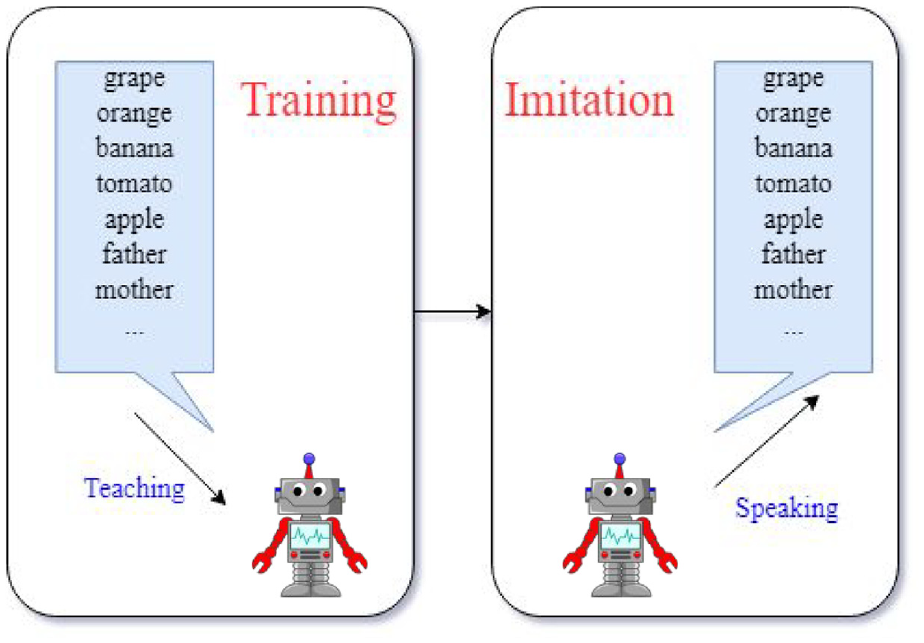
Concept of the proposed method.

Generally, conventional methods of voice generation input relevant parameters into a model and iteratively create a single audio signal according to those parameters, as illustrated in Figure 2(a). Because the same set of parameters can only represent the output of a single audio signal, the use of such a method enables only the continuous generation of the exact same audio signal and cannot therefore enhance the diversity and vividness of sounds. The method proposed in this article employs a thoroughly dissimilar logic to design a model. In a normal state, the intonation, emotions, and even timbre of human speech vary with time or situations. Therefore, even if the same sentence is continuously repeated during the same period of time, it is impossible for the collected audio signal to be completely similar every time. However, in related applications to robots, most employ the fixed text-to-speech (TTS) mode^26,27 technology to enable users to understand robots’ expressions by listening. Although TTS technology is increasingly maturing, and users can easily understand its content, the audio signals generated by TTS usually exhibit relatively flat intonation and generate the same audio signals each time they are played. Therefore, they are unable to produce a humanlike impression. However, the framework used in this article randomly generated a variety of audio signals with the same semantics by inputting a string of random variables, as illustrated in Figure 2(b).

Figure 2.

Comparison between (a) the conventional method and (b) the proposed method.

By means of the GAN special training method, researchers can generate audio signals with the same semantics—and that have never appeared in training data—from latent space interpolation. This also substantially enhances the diversity of the voice generation model and increases the realism when humans listen to robot sounds, thus strengthening the acceptance in human–machine interaction.

Proposed model with an autoencoder and GAN

This section is divided into two subtopics for discussion, the first of which is an introduction of the proposed model in this article. However, the optimizer performs a key role in the training process of the model, including its training speed, training results, and even whether the model can converge. Therefore, the second portion of the section focuses on the optimizer used in this article and explains the advantages of using this method.

The proposed model

The GAN model is primarily composed of a generator and discriminator, and its detailed functions are illustrated in Figure 3. Assuming that the data to be generated operate in a two-dimensional space, blue dots are used to indicate the real data distribution. Although the blue dots follow, admittedly, an unknown distribution, the researchers hoped to use the generator to generate a closely similar distribution to that of the real data, as represented by the orange dots in Figure 3. However, because the distribution mapped from latent space did not coincide initially, to facilitate the gradual coincidence of the distributions, a discriminator had been used to judge data authenticity. Therefore, following data generation by the generator, the discriminator judged the authenticity of the data, as demonstrated by the red dotted line.

Figure 3.

Functions of the generator and discriminator.

Figure 4 illustrates the changes in data distribution during training of the GAN model. Initially, because the data distribution generated by the generator differed considerably from the real data distribution, the discriminator easily differentiated authenticity. However, after several training, the data distribution generated by the generator conformed to that of the real data. Therefore, differentiating gradually became difficult for the discriminator. At the end, the data distribution generated by the generator nearly conformed to the real data distribution, which indicated that the generator generated data that are difficult for humans and the discriminator to differentiate in terms of authenticity. Consequently, the training was successful.

Figure 4.

Adversarial training process of GAN.

The system flowchart of the proposed denoise autoencoder with generative adversarial networks (DNAE-GAN) model is denoted in Figure 5. The model proposed in this article consists of two main stages. In the initial GAN training stage, the latent space distribution of the generated data greatly differs from that of the original data, and the discriminator lacks sufficient data for determining data authenticity. As the adversarial training process between the two deep neural networks progresses, the generated data distribution gradually becomes more similar to the original data distribution. After repeatedly conducting the training process, the latent space mapped by the generator gradually conforms to the original data. This indicates that the generator has learned how to generate the actual data. At this stage, the discriminator cannot differentiate between the generated data and original data, thus signifying completion of the GAN training process.

Figure 5.

System flowchart of the DNAE-GAN.

After completing the GAN training, the audio created by the generator is capable of fooling the discriminator but still exhibits excessive noise. The proposed method employed a denoise autoencoder to address this problem by connecting the trained generator to the autoencoder to fix the generator and reduce the amount of noise while fine-tuning it. The initial training process revealed that the distribution of the generated data was substantially different from that of the original data. Throughout the training process, the generated data gradually conformed to the original data until the differences between the generated data and the original data were minimal, indicating that the autoencoder training was successful.

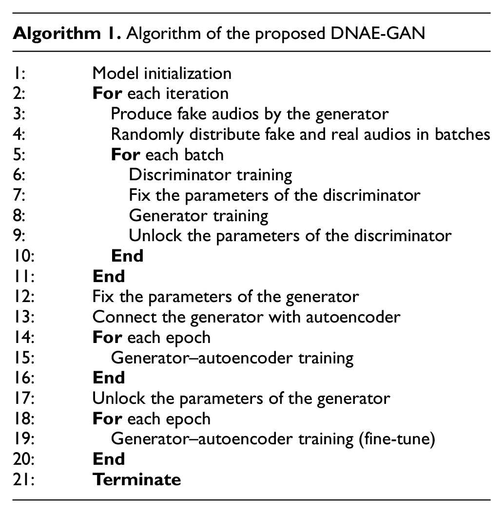
The detailed training process is illustrated in Algorithm 1. Following the aforementioned training process, the proposed DNAE-GAN generated the corresponding various audios based on the inputted random variables. Essentially, after the first generator–autoencoder training process, the quality of the generated audio was already evidently improved and acceptable. However, fine-tune training was still executed for better performance.

Figure 6 displays the framework for the proposed model with DNAE-GAN. Figure 6 indicates that random variables are directly input into the generator, whereas the generator’s output is a fake audio. In the same training batch, the fake audio and original audio enable the discriminator to perform training with the aim of determining data authenticity. After training of the entire GAN architecture, the discriminator that the generator was originally connected to was removed, and the generator was connected to the autoencoder, which was composed of an encoder and decoder. Following completion of the GAN architecture training, due to the excessive noise of the generator, the final output was based on the combined architecture of the generator and autoencoder, rather than on the output result of the generator alone. This area is also where this article differs from typical GAN architectures.

Figure 6.

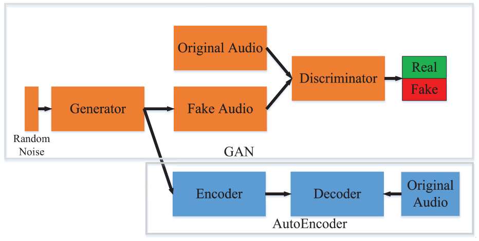
Architecture of the proposed DNAE-GAN.

The operational concept of the denoise autoencoder proposed in this article is illustrated in Figure 7. Generally, the training method of an autoencoder is unsupervised learning. Therefore, the input and output signals usually generate themselves. The feature maps generated by some autoencoders after passing through an encoder can also be regarded as the compression-coded result of its input signal. An autoencoder also possesses the function of data compression. In this article, however, because the objective of the autoencoder was to denoise, the input and output data were regarded as distinct data. During the training of the denoise autoencoder, input data comprised audio signals with noise, whereas output data comprised signals without noise. Consequently, because the voice generated by the generator had noise, the output of the generator was directly docked to the autoencoder’s input. The autoencoder output was expected to be the same as the original audio file, that is, a voice without noise. During training, however, the researchers expected that the audio file on the output end of the autoencoder would be randomly selected. The goal was to maintain diversity in the output of the model proposed in this article, rather than exhibiting a bias toward certain audio files. This was also key in the autoencoder training process.

Figure 7.

Function of the denoise autoencoder.

Algorithm 1. Algorithm of the proposed DNAE-GAN
1:	Model initialization
2:	For each iteration
3:	Produce fake audios by the generator
4:	Randomly distribute fake and real audios in batches
5:	For each batch
6:	Discriminator training
7:	Fix the parameters of the discriminator
8:	Generator training
9:	Unlock the parameters of the discriminator
10:	End
11:	End
12:	Fix the parameters of the generator
13:	Connect the generator with autoencoder
14:	For each epoch
15:	Generator–autoencoder training
16:	End
17:	Unlock the parameters of the generator
18:	For each epoch
19:	Generator–autoencoder training (fine-tune)
20:	End
21:	Terminate

The DNAE-GAN architecture proposed in this article is divided into a discriminator, generator, and autoencoder. The discriminator comprised six layers, each of which uses MLP architecture, as illustrated in Figure 8. This architecture is characterized by the fact that the neurons between each layer are fully connected. In the DNAE-GAN architecture, the discriminator is connected after the generator, that is, the generator’s output is the discriminator’s input. Therefore, the discriminator’s input is a one-dimensional audio signal that has been flattened. Because the primary role of the discriminator is to differentiate the authenticity of the generated data, its output can be expressed using only one neuron. Although the number of its input neurons exceeds 4000, only one output exists. Therefore, in the design of each layer, the number of neurons is gradually decreased to avoid a sudden reduction of neurons in the last layer, which would result in poor model training.

Figure 8.

Architecture of the discriminator.

The architecture of the generator is similar to that of the discriminator as presented in Figure 9. A major reason for this similarity is that, during model training, if the architectures of the generator and discriminator differ excessively, their abilities exhibit a disproportionate gap, which leads to difficulty in model training and thus results in convergence difficulty. Therefore, the generator in this article also comprised six layers and primarily used an MLP-based architecture. The generator differs from the discriminator in terms of input. Because it is latent space, the generator’s input is a random variable. In this article, a one-dimensional random variable with a length of 100 was selected as the size of the latent space. The length of 100 was selected because latent space is the starting position of data mapping. If it is excessively large, an exceedingly lengthy amount of time and large amount of data are required to fill completely the latent space during GAN training. Such a practice causes slowed training progress and convergence difficulty. However, an excessively small size causes the GAN output to have exceedingly low recognition. Therefore, after several experiments, the latent space of the generator in this article was suitably selected as 100. Because the generator’s output was an audio signal and had to be directly input into the discriminator, the length of the generator’s output had to correspond with that of the discriminator’s input to complete training. The length of the generator’s output was thus set to 4000.

Figure 9.

Architecture of the generator.

Another focus in this article was the autoencoder, which is the key to eliminating noise from the generator’s audio signal output. The autoencoder architecture is illustrated in Figure 10. Because the autoencoder undergoes unsupervised training, no certain answers exist during autoencoder training. The output and input of the autoencoder are usually the same size, and after inputting the same data, the primary objective is for the expected output value to be the same as the input value. Accordingly, the input and output of the autoencoder in this article were both set to 40,000. Another crucial feature of the autoencoder is that it contains an encoder and a decoder. The encoder and decoder are symmetric, that is, the numbers of layers are the same, as well as the numbers of neurons per layer. Moreover, the number of neurons in the encoder decreases, whereas that in the decoder increases. Because of the decrementing and incrementing process of the autoencoder input, the original, noisy audio signal can be changed into a purer audio signal during training.

Figure 10.

Architecture of the denoise autoencoder.

In this article, the activation function of all models uses a variant of the rectified linear unit (ReLU), Leaky ReLU. Generally, the activation functions of early neural networks primarily consist sigmoid and tanh, the formulas of which are presented in equations (1) and (2). In recent years, an increasing number of researchers have discovered that the use of ReLU can effectively overcome gradient vanishing. Its formula is presented in equation (3). The concrete reason for this effectiveness is that the functions of sigmoid and tanh are close to the saturated zone, and their values after differentiation are near 0, which corresponds to gradient vanishing. As a result, updated messages cannot be transmitted using back propagation. After experiment, in addition to solving gradient vanishing, the use of ReLU was reported to mitigate overfitting. However, issues were also encountered in the use of ReLU. For example, in areas where the range of values is less than 0, its output value is constantly 0. This neuron can thus be considered as no longer having effect. Related research revealed that, during training, it is difficult to reactivate neurons that have lost effect, which is well-known as the “dead ReLU problem.” Leaky ReLU was devised to solve this issue, and its formula is presented in equation (4). Its most prominent feature is that its outputs continue to have value despite the range being negative. Although changes are minimal, neurons do not necessarily die completely. Therefore, Leaky ReLU possesses the advantages of ReLU yet can maintain neuron activity. This is the primary reason why this article employed Leaky ReLU. These four activation functions are illustrated in Figure 11. The figure indicates that the sigmoid is between 0 and 1, whereas the tanh is between −1 and 1. ReLU ranges from 0 to positive infinity, whereas Leaky ReLU can be both infinitely small and large. Although Leaky ReLU exhibits a gentler gradient for negative values, it retains its value, which enables neurons to continue activation without premature death

$$\mathrm{Sigmoid}(x)=\frac{1}{1+e^{-x}}$$

(1)

$$\mathrm{Tanh}(x)=\frac{2}{1+e^{-2x}}-1$$

(2)

$$\mathrm{ReLU}(x)=max(0,x)$$

(3)

$$\mathrm{LeakyReLU}(x)=\{\begin{array}{c}x\mathrm{if}x\ge 0\hfill \\ \multicolumn{1}{c}{\alpha x\mathrm{if}x<0}\end{array}$$

(4)

Figure 11.

Activation functions: (a) sigmoid, (b) Tanh, (c) ReLU, and (d) Leaky ReLU.

Optimizer

Because a neural network is composed of several weights, the training of a neural network is based on the adjustment of its weights. The optimizer is crucial in the process of adjusting weights. A neural network’s training speed, performance after training, and even convergence capability is closely related to the choice of optimizer. Generally, if the parameter of a neural network at time t is θ_t, the method by which its parameter is updated the next moment can be expressed by equations (5)–(7)

$${\theta }_{t+1}={\theta }_t+\mathrm{\Delta }{\theta }_t$$

(5)

$$\mathrm{\Delta }{\theta }_t=-\eta g_t$$

(6)

$$g_t=\frac{\partial f({\theta }_t)}{\partial {\theta }_t}$$

(7)

In equation (6), Δθ_t represents the correction of the parameter, and η represents the learning rate. Although a greater value here indicates faster learning, it may also result in the consequence of impossible convergence. However, if η is too small, although the training process becomes more exact, training efficiency becomes considerably low. Therefore, the size of the η value plays a crucial role in neural network training. In equation (7), g_t represents the gradient at time t, which can be calculated by the partial differentiation of the objective function f(θ_t) from the parameter θ_t.

Most basic optimizers often encounter oscillation near optima during the training process because of improper learning rate configuration and cannot effectively converge to an optimal solution. The Momentum method was conceived to solve the aforementioned issue and is presented in equation (8)

$$\mathrm{\Delta }{\theta }_t=\rho \mathrm{\Delta }{\theta }_{t-1}-\eta g_t$$

(8)

The aforementioned formula suggests that parameter updates in Momentum are related to parameter updates in the previous moment, where ρ is a constant used to control the effect of Δθ_t-1. Because each parameter update is related to the previous moment, and earlier parameter updates have smaller effects on current parameter updates, Momentum can effectively alleviate the oscillation of parameter correction during neural network training.

The optimizer employed in this article is the Adaptive Learning Rate Method (AdaDelta). ²⁸ The computation of AdaDelta was revised from that of the Adaptive Subgradient Methods (AdaGrad). ²⁹ The AdaGrad algorithm is presented in equation (9)

$$\mathrm{\Delta }{\theta }_t=\frac{-\eta }{\sqrt{\sum _{\tau =1}^t{g}_{\tau }^2}}{g}_t$$

(9)

The aforementioned formula reveals that parameter updates in AdaGrad are related to the accumulated sum of the gradient each time. Because the sums of squares of gradients are positive, when the number of iterations increases, the parameter updates decrease. Although the value of the learning rate has not changed, this method indirectly controls the learning rate of the neural network and optimizes its learning outcome.

The AdaDelta method takes into account more detailed factors, and its formula is primarily provided in equations (10)–(13)

$$E[g^2{]}_t=\rho E[g^2{]}_{t-1}+(1-\rho )g_t^2$$

(10)

$$E[\mathrm{\Delta }{\theta }^2{]}_t=\rho E[\mathrm{\Delta }{\theta }^2{]}_{t-1}+(1-\rho )\mathrm{\Delta }{\theta }_t^2$$

(11)

$$\mathrm{RMS}[g{]}_t=\sqrt{E{[g^2]}_t+\epsilon }$$

(12)

$$\mathrm{\Delta }{\theta }_t=\frac{-\mathrm{RMS}{[\mathrm{\Delta }\theta ]}_{t-1}}{\mathrm{RMS}{[g]}_t}{g}_t$$

(13)

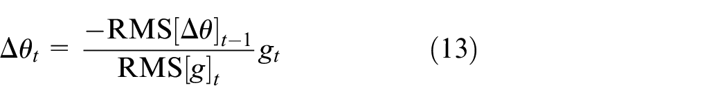
where E[g²] _t is the accumulated gradient and E[θ²] _t is the accumulated updates. From the aforementioned formula, all parameter updates are evidently related to the accumulated gradient and accumulated updates. The factors considered are more detailed, and a study ²⁸ presented a detailed comparison of its performance.

The choice of loss function of a neural network is also highly crucial. Because the learning algorithm examined in this article was not classification, and the discriminator needed only to identify data authenticity, the model proposed in this article employed mean square error (MSE) to calculate loss value. The formula for MSE is presented in equation (14)

$$\mathrm{MSE}=\frac{\sum _{n=1}^N{(y_n-{\hat{y}}_n)}^2}{N}$$

(14)

where $y_n$ is the desired value and ${\hat{y}}_n$ is the estimated value. The calculation of the MSE enables the neural network to further understand the gap between the current and ideal values, thus enabling the optimizer to perform parameter optimization.

Experimental results

This section is divided into two sections. The first section introduces the DNAE-GAN training data, and the second section presents the DNAE-GAN experimental results.

Training data

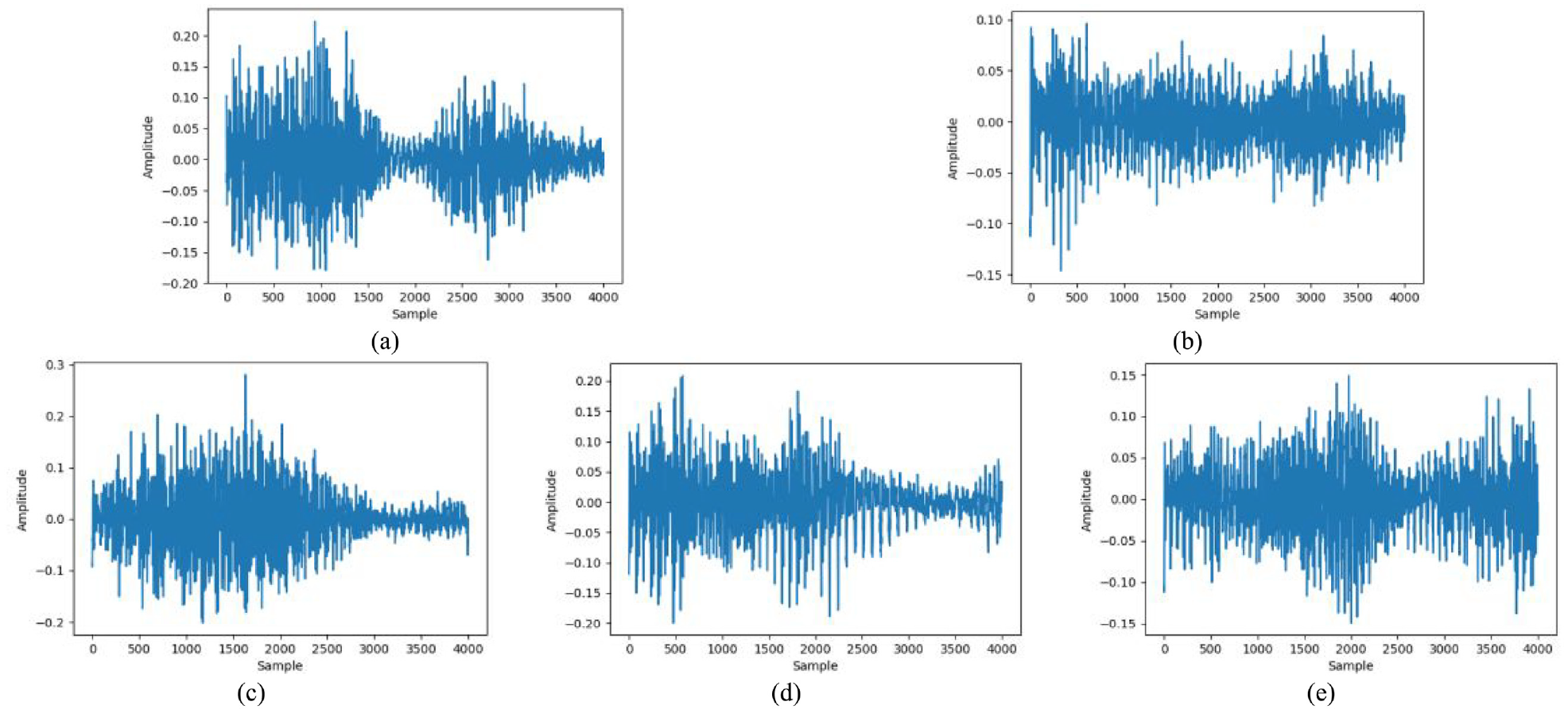
The training data contained 300 audio samples, which are separated into five categories according to the fruit word pronounced in each sample. Each category consists of 60 audio files. Figure 12(a)–(e) displays a sample of the training data for each fruit word. Each audio file was 4000 ms and 8000 Hz. The file amplitudes ranged between −1 and 1.

Figure 12.

Training data for the DNAE-GAN: (a) apple, (b) banana, (c) grape, (d) orange, and (e) tomato.

Experimental results

Figure 13(a) displays the discriminator loss value, which is fluctuating because the discriminator is competing with the generator, as shown in Figure 13(b), and a comparison of the two figures show that the loss values of the discriminator and the generator loss value, as denoted in Figure 13(b), are nearly the identical. Because of the relationship between GAN training characteristics, the generator and discriminator continuously engage in competitive learning. Therefore, it is normal for their loss values to fluctuate constantly. The experimental results revealed that during GAN training, the special training method enabled the discriminator and generator to compete with and learn from each other, which resulted in fluctuating loss value that tended to cause unstable training. Accordingly, the GAN training process was difficult, which may have led to an unsatisfactory generator output. As indicated in Figure 13(c), the autoencoder loss value was continually decreasing. After numerous experiments, the autoencoder training was proven to achieve convergence in approximately 1000 epochs. It also demonstrates the feasibility of the proposed method. The input of the autoencoder (AE) was the audio with noise from the generator, and the original random audio signal was used at the output end of the generator as its label. Furthermore, AE is a type of unsupervised learning, and its loss value was discovered to steadily decline with increasing training epoch during the AE training process. Therefore, the AE was determined to have a high training stability and could thus assist the generator in producing favorable results. Figure 14 displays the excessive noise exhibited by the generated voice after the generator has undergone GAN training. Even though the original voice could sometimes be heard within the generated voice, the results were still unsatisfactory. Therefore, the proposed method connected the trained generator to the autoencoder for further training. The generator was fixed during the second training process, and the final training results are shown in Figure 15, which indicates that the noises have been eliminated and the original voice can be clearly heard in the generated voice. Thus, the experimental results prove the feasibility of the DNAE-GAN training method.

Figure 13.

Learning curve of the proposed DNAE-GAN: (a) discriminator, (b) generator, and (c) autoencoder.

Figure 14.

Generated results of the GAN: (a) apple, (b) banana, (c) grape, (d) orange, and (e) tomato.

Figure 15.

Generated results of the DNAE-GAN: (a) apple, (b) banana, (c) grape, (d) orange, and (e) tomato.

The whole experimental video can be accessed using the following link: https://youtu.be/77-67bxthYM (accessed 13 October 2019). The aforementioned experimental videos revealed that using the conventional GAN approaches to synthesize audio signals produced extremely loud noises, which nearly obscured the original audio that the generator aimed to present. This confirmed the low feasibility of using only GANs for audio synthesis. Thus, the author proposed using the DNAE approach and input the audio produced by the original generator into the AE to filter the noises. The experimental video indicated that the AE improved the audio from being nearly indistinguishable to being clear and recognizable. This again verified the feasibility of the method proposed in this article.

Discussions

Generally, related applications of GAN have focused on image applications, with only few applications in audio signals. This is partially because an image is a two-dimensional signal, whereas sound is a one-dimensional signal, and its analysis and feature extraction are more difficult to perform. For voice generation, a sample quantity of 4000 is sufficient. Furthermore, to accurately generate voice, the error each time cannot be too high, or noise is easily generated. Even a small amount of noise is clearly heard in audio signals. Therefore, a certain difficulty existed in the subject of this article.

Following the addition of the denoise autoencoder, noise was significantly reduced. Although a slight amount of noise remained upon careful listening, the results were substantially enhanced compared with those without the addition of the denoise autoencoder, and they were within an acceptable range for human hearing. The architecture proposed in the model of this article does not require a lot of computing resources and is not composed of large parameter sizes. In contrast to several other models that require considerable amounts of computing resources to achieve favorable performance, the method proposed in this article is more efficient and feasible. Furthermore, if a model is excessively large, compared with its own weight, its computing resources will be relatively weak when it is applied to mobile robots. The use of an excessively large model results in the inability to promptly respond to the user. Therefore, in consideration of computing resources, the model in this article was designed to achieve the most favorable effect using the minimum computing resources.

The model proposed in this article may be used for any voice data. To verify the results of the diverse experiments conducted, five words were adopted to perform experiments. The model generated voices beyond these five words. In the future, training can be conducted on multiple words, and even entire sentences, which will enable neural networks to generate more diverse and richer voices. Few studies have investigated the use of the GAN type for voice generation. The architecture in this article is also novel and promotes a new wave of research in the future.

However, to use GANs for audio generation, many current technologies merit in-depth discussion. For example, from the literature^30,31 and the use of adversarial AEs to reduce the data dimension, the experimental results revealed that using an adversarial AE yielded a superior result to using a conventional AE. Deng et al. ³² used model-based Q-learning together with Gaussian process regression and knowledge transfer technology to teach skills to robots. Ke et al. ³³ employed Wasserstein GANs to perform automatic image annotation; the Wasserstein GANs were more stable than the conventional GAN architecture for image processing, could prevent divergence in training, and achieved high performance. Collaborative filtering is a critical technology for the internal processing of recommendation systems. Wang et al. ³⁴ used novel AE training on collaborative filtering to attain satisfactory experimental results. In addition, AEs have evolved into various other structures. For example, Xu et al. ³⁵ used a stacked AE to process social image understanding problems, and its superior effectiveness was verified in the experiment. Elhami and Weber ³⁶ used a convolutional AE for the feature extraction of audio signals, and the experimental results verified that the AE using CNN architecture yielded excellent performance on speech signals. Furthermore, Otto and Rowley ³⁷ used linearly recurrent AE networks that changed the original AE into the form of an RNN, whose characteristics enabled the modified AE architecture to achieve superior performance in time series analysis. Guo et al. ³⁸ discussed multimodal representation learning in detail. The encoder–decoder model and GAN-related technologies mentioned in the study have been studied, discussed, and constantly improved by subsequent studies, which indicates that these two technologies will be a key research direction in the future.

Conclusion

This article proposes a voice generation model that employs a combination of denoise AE and GANs as its fundamental operation mechanism, resolving the lack of diversity in LPC-generated audio. The experimental results indicated that general voices generated by a GAN framework exhibit excessive noise. To solve these problems, this model employs an AE for denoising, and the proposed method adopted a unique training method to ensure AE operation efficiency. After fixing the generator parameters, the generator was connected to the AE for training, thereby removing noise in the generated sounds. The experimental results indicate that the DNAE-GAN method demonstrated outstanding performance and also prove the feasibility of the proposed method. The method proposed in this study does not require a huge neural network architecture; nevertheless, it exhibits relatively high performance among small neural network architectures studied in research. Although it may not be able to obtain clearer results than those obtained by a huge neural network, the reduced computational complexity may increase the feasibility of this method on embedded systems. The success of this experiment signified that using GAN and AE architectures for audio synthesis in academic research is indeed feasible and a direction worth studying. However, the method proposed in this article still has limitations because a large number of speech samples may gradually overwhelm the original GAN. Therefore, on the basis of the proposed method, future research may improve GAN and AE architectures in depth to achieve better audio synthesis effects. In addition, the proposed method can be applied in the audio generation for service robots to make a robot’s voice more vivid and of closer resemblance to that of humans.