Sage Journals: Discover world-class research

Abstract

In this article, versatile video coding, the next-generation video coding standard, is combined with a deep convolutional neural network to achieve state-of-the-art image compression efficiency. The proposed hierarchical grouped residual dense network exhaustively exploits hierarchical features in each architectural level to maximize the image quality enhancement capability. The basic building block employed for hierarchical grouped residual dense network is residual dense block which exploits hierarchical features from internal convolutional layers. Residual dense blocks are then combined into a grouped residual dense block exploiting hierarchical features from residual dense blocks. Finally, grouped residual dense blocks are connected to comprise a hierarchical grouped residual dense block so that hierarchical features from grouped residual dense blocks can also be exploited for quality enhancement of versatile video coding intra-coded images. Various non-architectural and architectural aspects affecting the training efficiency and performance of hierarchical grouped residual dense network are explored. The proposed hierarchical grouped residual dense network respectively obtained 10.72% and 14.3% of Bjøntegaard-delta-rate gains against versatile video coding in the experiments conducted on two public image datasets with different characteristics to verify the image compression efficiency.

Keywords

Image compression coding artifact reduction CNN deep learning VVC

Introduction

Image compression is a crucial technology for rich multimedia services over the Internet; it allows viewing high-quality natural and synthetic images created by an expert photographer on a web browser; it allows sharing tremendous number of photos taken by users through a social network service; in addition, an intuitive user interface based on compressed images allows users to explore other multimedia services. Highly efficient image compression can increase user satisfaction with multimedia services on the Internet by reducing image loading time or enabling higher quality image viewing. Also, it can provide a seamless multimedia service even in severe network environment. Therefore, even though image compression such as JPEG, WebP,¹ and BPG² already exists, higher image compression efficiency is still required.

Image compression using deep neural network (DNN) has become one of the emerging research fields due to its potential for significant improvement of compression efficiency over handcrafted algorithms. Joint Photographic Experts Group (JPEG) of ISO/IEC JTC1/SC29/WG1 and ITU-T SG16 is exploring DNN-based image compression technology for JPEG-AI.^3,4 To improve image compression efficiency using a dedicated DNN, it can be end-to-end trained to efficiently code latent variables using a probability distribution model.^5–9 Recent works^8,9 in this type of approach show superior performance than BPG which is compatible with high-efficiency video coding (HEVC) intra coding, for both peak signal-to-noise (PSNR) and multi-scale structural similarity (MS-SSIM).¹⁰ As another type of approach to improve image compression efficiency, a DNN can be used to improve the quality of an image that has already been reconstructed after compression. Joint Video Experts Team (JVET), jointly formed by ISO/IEC Moving Picture Experts Group (MPEG) and ITU-T Video Coding Experts Group (VCEG), is currently standardizing the next-generation video compression technology, versatile video coding (VVC).¹¹ VVC has a requirement to improve the compression efficiency of existing HEVC¹² by more than 30% and 50% for the same perceptual quality depending on use-cases.¹³ This work focuses on quality enhancement of VVC intra-coded images to maximize the image compression efficiency. There are three main contributions of this work:

VVC intra coding is combined with the proposed DNN-based compression artifact removal method to obtain a state-of-the-art image compression efficiency. Experimental results show that substantial quality enhancement is achieved with the proposed method for a wide bitrate range.

Hierarchical grouped residual dense network (HGRDN) architecture is proposed to efficiently remove artifacts from VVC intra coding. Combinations of feature fusion in different architectural levels are explored to determine the overall HGRDN architecture.

Non-architectural aspects affecting the training efficiency and the performance of HGRDN, such as size of the training image patch and number of the convolutional filters, are investigated. An effective learning rate decaying strategy is also introduced to adaptively adjust the learning rate throughout the training period of HGRDN.

The remainder of this article is organized as follows. Section “Related works” provides brief introductions to VVC intra coding and DNN-based image quality enhancement. Section “Proposed method” presents the details of our proposed HGRDN in each architectural level. Section “Results and discussions” provides experimental results and discussions. Finally, we conclude our work in section “Conclusion.”

Related works

VVC intra coding

VVC supports a 128 × 128 Coding Tree Unit (CTU) size that is extended from the maximum CTU size of HEVC, 64 × 64. A more sophisticated block partitioning scheme, which extends HEVC’s quadtree to quadtree plus binary tree and ternary tree (QTBTTT), is adopted for VVC. Figure 1(a) depicts an example of QTBTTT block partitioning of VVC. VVC also extends the maximum transform size from 32 × 32 to 64 × 64. Furthermore, mode-dependent non-separable secondary transforms and explicit multiple core transforms are adopted for VVC intra-frame coding. Although these changes are not directly related to intra prediction, they give VVC intra-frame coding a substantial coding gain compared to HEVC. Following are the coding tools adopted for VVC to improve intra-prediction accuracy:¹⁴

Sixty-seven intra-prediction modes (refer to Figure 1(b));

Wide-angle intra prediction for non-square blocks;

Block size and mode-dependent four-tap interpolation filter;

Position-dependent intra-prediction combination;

Cross-component linear model intra prediction;

Multi-reference line intra prediction;

Intra sub-partition.

It is reported that VVC has achieved 23.14% of Y-PSNR Bjøntegaard delta (BD)-rate gain on average when the VVC test model (VTM)¹⁵ is compared with the HEVC test model (HM)¹⁶ in all intra-coding conditions.¹⁷

Figure 1.

(a) An example of QTBTTT block partitioning of VVC; (b) 67 intra-prediction modes of VVC. Both (a) and (b) are copied from Chen et al.¹⁴

DNN-based image quality enhancement

DNNs are being actively studied for recent years achieving great success on image restoration tasks such as image super resolution (SR), denoising, inpainting, and dehazing. The DNNs for such tasks have similar design considerations, thus they are affecting each other’s design and rapidly improving the performance for overall image restoration tasks. Enhancing the quality of compressed images and videos is a task to remove compression artifacts, which essentially falls into the same category with denoising, and DNN-based approaches are driving the performance improvement for this research field. Dong et al.¹⁸ introduced a DNN named artifact reduction convolutional neural network (AR-CNN) that is inspired by well-known super-resolution CNN (SRCNN)¹⁹ for image SR and successfully reduced JPEG artifacts. After that, following works^20–22 introduced DNNs with improved performance for JPEG artifact reduction.

The efforts were not limited to the traditional JPEG image codec; DNNs combined with a recent video codec HEVC for compression artifact reduction were also introduced. Dai et al.²³ achieved a 4.6% average BD-rate gain by post-filtering HEVC intra-coded frames with variable-filter-size residue-learning CNN (VRCNN) which uses multiple convolutional filer sizes. Soh et al.²⁴ introduced a DNN with temporal branches where the network extracts features from neighboring frames for artifact removal of the image patch in the current frame. This work achieved a 0.23-dB average PSNR gain by post-filtering HEVC frames encoded in random access (RA) condition; however, the gain was limited only for low bitrates. Yang et al.²⁵ proposed quality-enhanced CNN (QE-CNN) which mainly consists of two sub-networks, QE-CNN-I and QE-CNN-P, dedicated for HEVC intra-mode and inter-mode distortions, respectively. This one achieved an 11.06% average BD-rate gain when HEVC I and P frames are post-filtered with the dedicated sub-networks.

Several DNNs applied for VVC artifact reduction were introduced more recently. Lu et al.²⁶ proposed a DNN based on residual blocks in multiple spatial scales, and Cho et al.²⁷ applied grouped residual dense network (GRDN) that showed an excellent image denoising performance in Kim et al.²⁸ Both Lu et al.’s²⁶ and Cho et al.’s²⁷ models work as post-filters of VVC intra coding to obtain improved image compression efficiency. Cho et al.²⁷ achieved a superior performance over Lu et al.²⁶ in terms of PSNR and mean opinion score (MOS).²⁹ This work exploits the previous work²⁷ as a base model and extends it in different architectural levels to find out a better architecture for compression artifact reduction of VVC intra-coded frames.

Proposed method

In this section, the architecture of HGRDN is introduced in detail. HGRDN has top, middle, and bottom architectural levels each of which respectively determines the hierarchical grouped residual dense block (HGRDB), grouped residual dense block (GRDB), and residual dense block (RDB) sub-architectures. We introduce the HGRDN architectural levels in top-to-bottom order.

Top-level HGRDN architecture with HGRDB sub-architectures

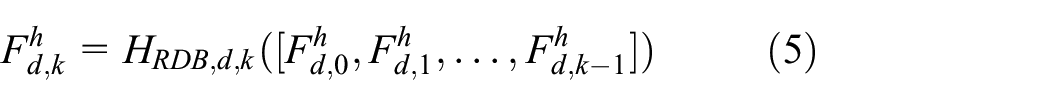
HGRDN consists of six parts in top-level: input feature extraction, down-sampling, an HGRDB which consists of GRDBs, up-sampling, a convolutional block attention module (CBAM), and global residual restoration. Figure 2 illustrates the top-level HGRDN architecture with three HGRDB sub-architectures—Serial, Merged, and Dense—that differ from each other depending on how GRDBs in an HGRDB are connected to each other. Figure 2(a) shows the top-level HGRDN architecture with Serial HGRDB sub-architecture. It should be noted that Serial herein means the HGRDB has a number of serialized GRDBs in it, as shown in the gray box in Figure 2(a). The first convolutional layer of HGRDN depicted as Conv in Figure 2 extracts a feature map $F_{0}$ from the input image $I_{A}$ , which is $F_{0} = H_{I 2 F} (I_{A})$ , where $H_{I 2 F} (\cdot)$ denotes 3 × 3 convolutional operation with stride equal to 1. $F_{0}$ is then down-sampled so that both width and height of $F_{0}$ to be half in resulting feature map $F_{0}^{h}$ , without changing the depth; it can be written as $F_{0}^{h} = H_{DS} (F_{0})$ , where $H_{DS} (\cdot)$ denotes 4 × 4 convolutional operation with stride equal to 2. Down-sampling $F_{0}$ to $F_{0}^{h}$ allows HGRDN to have more internal layers resulting in a deeper HGRDN and it also allows the HGRDN to accept larger images within a given amount of memory. $F_{0}^{h}$ is fed into the first GRDB in Serial HGRDB as shown in Figure 2(a). The output of dth GRDB in Serial HGRDB is

\begin{matrix} F_{d}^{h} = H_{GRDB, d} (F_{d - 1}^{h}) \\ = H_{GRDB, d} (H_{GRDB, d - 1} (\dots (H_{GRDB, 1} (F_{0}^{h})) \dots)) \end{matrix}

(1)

where $H_{GRDB, d}$ denotes the operation of the dth GRDB in Serial HGRDB, which is addressed in section “Middle-level HGRDN architecture with GRDB sub-architectures.” The feature map $F_{D}^{h}$ from the last GRDB in Serial HGRDB is up-sampled to its original width and height, which can be written as $F_{D} = H_{US} (F_{D}^{h})$ , where $H_{US}$ denotes 4 × 4 transposed convolutional operation with stride equal to 2. To make HGRDN more attentive on significant features to reduce VVC artifact, the channel and spatial attention mechanism introduced in Woo et al.³⁰ is adopted. To this end, $F_{D}$ is fed into CBAM in Figure 2 to obtain the refined feature map, $F_{A}$ , that can be written as $F_{A} = H_{CBAM} (F_{D})$ , where $H_{CBAM}$ denotes the composite operation of the CBAM in Woo et al.³⁰ The last Conv in HGRDB adjusts the number of channels in $F_{A}$ to that of the output image; it can be written as $F_{I} = H_{F 2 I} (F_{A})$ , where $H_{F 2 I} (\cdot)$ denotes 3 × 3 convolutional operation with stride equal to 1. Utilizing benefits of global residual learning, $F_{I}$ is then added to the input image $I_{A}$ to obtain the final output of HGRDN; $I_{AF} = F_{I} + I_{A}$ , where $I_{AF}$ is the output image of HGRDN.

Figure 2.

Top-level HGRDN architecture with different HGRDBs: (a) Serial HGRDB and (b) Merged and Dense HGRDBs. In (b), Merged HGRDB only includes solid arrows, while Dense HGRDB includes both solid and dashed arrows.

Figure 2(b) shows the top-level HGRDN architecture with Merged and Dense HGRDB sub-architectures. The difference between Serial and the other two HGRDB sub-architectures is the connectivity between GRDBs that can be noted by comparing the gray boxes in Figure 2(a) and (b). The output of dth GRDB $F_{d}^{h}$ in Merged HGRDB can be written as same as $F_{d}^{h}$ in equation (1). Meanwhile, Dense HGRDB exploits hierarchical features by concatenating the feature map from a GRDB to all the following GRDBs’ input, which is shown with dashed arrows in Figure 2(b). $F_{d}^{h}$ in Dense HGRDB is

F_{d}^{h} = H_{GRDB, d} ([F_{0}^{h}, F_{1}^{h}, \dots, F_{d - 1}^{h}])

(2)

where $H_{GRDB, d}$ denotes the operation of the dth GRDB in Dense HGRDB and $[F_{0}^{h}, F_{1}^{h}, \dots, F_{d - 1}^{h}]$ refers to the concatenation of the feature maps. The depth of $F_{d}^{h}$ is designed to be G, also kwon as growth rate,³¹ in Dense HGRDB. To exploit hierarchical features, the feature map of each GRDB in Merged and Dense HGRDBs is fused together with the feature maps of the other GRDBs. More specifically, the feature maps $F_{0}^{h}, F_{1}^{h}, \dots, F_{D}^{h}$ in Merged and Dense HGRDBs are concatenated and fed into a 1 × 1 convolutional layer as illustrated in Figure 2(b) with solid arrows; it can be written as

F_{GF}^{h} = H_{GF}^{h} ([F_{0}^{h}, F_{1}^{h}, \dots, F_{D}^{h}])

(3)

where $H_{GF}^{h}$ is the function of the 1 × 1 Conv in Figure 2(b) to adjust the output depth. To utilize the benefit of local residual learning, $F_{GF}^{d}$ in Merged and Dense architectures is then added to $F_{0}^{h}$ to obtain the HGRDN output $F_{DF}^{h}$ , which is $F_{DF}^{h} = F_{GF}^{h} + F_{0}^{h}$ .

Middle-level HGRDN architecture with GRDB sub-architectures

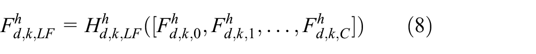
GRDB consists of three parts: an input convolutional layer, RDBs, and local residual restoration. Figure 3 illustrates the middle-level HGRDN architecture with two GRDB sub-architectures, Merged and Dense, that differ from each other depending on how RDBs in a GRDB are connected to each other. The input convolutional layer of dth GRDB that is depicted as Conv-in in Figure 3 adjusts the depth of input $F_{d - 1}^{h}$ to G in the resulting feature map $F_{d, 0}^{h}$ so that GRDBs in a Dense HGRDB can accept input $F_{d - 1}^{h}$ regardless of the input depth; that is, $F_{d, 0}^{h} = H_{DH} (F_{d - 1}^{h})$ where $H_{DH} (\cdot)$ denotes 3 × 3 convolutional operation with stride equal to 1. It should be noted that the Conv-in is not necessary for those GRDBs in a Serial or a Merged HGRDB. $F_{d, 0}^{h}$ is then fed into the first RDB, and the output of kth RDB in Merged GRDB is

\begin{matrix} F_{d, k}^{h} = H_{RDB, d, k} (F_{d, k - 1}^{h}) \\ = H_{RDB, d, k} (H_{RDB, d, k - 1} (\dots (H_{RDB, d, 1} (F_{d, 0}^{h})) \dots)) \end{matrix}

(4)

where $H_{RDB, d, k}$ denotes the operation of the kth RDB in dth Merged GRDB which will be de addressed later in section “Bottom-level HGRDN architecture with RDB sub-architecture.” Meanwhile, Dense GRDB exploits hierarchical features in the same way as Dense HGRDB does, which is shown with dashed arrows in Figure 3. The output of kth RDB in Dense GRDB is

F_{d, k}^{h} = H_{RDB, d, k} ([F_{d, 0}^{h}, F_{d, 1}^{h}, \dots, F_{d, k - 1}^{h}])

(5)

where $H_{RDB, d, k}$ denotes the operation of the kth RDB in dth Dense GRDB. The depth of $F_{d, k}^{h}$ is designed to be G in Dense GRDB. The feature maps $[F_{d, 0}^{h}, F_{d, 1}^{h}, \dots, F_{d, K}^{h}]$ in both Merged and Dense GRDBs are concatenated and fed into a 1 × 1 convolutional layer as illustrated in Figure 3 with solid arrows; it can be written as

F_{d, LF}^{h} = H_{d, LF}^{h} ([F_{d, 0}^{h}, F_{d, 1}^{h}, \dots, F_{d, K}^{h}])

(6)

where $H_{d, LF}^{h}$ is the function of the 1 × 1 Conv in Figure 3 to adjust the output depth. $F_{d, LF}^{h}$ is then added to $F_{d, 0}^{h}$ to obtain the GRDB output $F_{d}^{h}$ , which is $F_{d}^{h} = F_{d, LF}^{h} + F_{d, 0}^{h}$ .

Figure 3.

Middle-level HGRDN architectures with Merged and Dense GRDBs; Merged GRDB only includes solid arrows, while Dense GRDB includes both solid and dashed arrows; the Conv-in is only valid for GRDBs in a Dense HGRDB.

Bottom-level HGRDN architecture with RDB sub-architecture

Figure 4 illustrates the bottom-level HGRDN architecture with RDB sub-architecture. In this work, the RDB introduced by Zhang et al.³² is used with a minor modification. RDB in this work consists of three parts: an input convolutional layer, convolutional layers with rectified linear unit (ReLU) activation function, and local residual restoration. The input convolutional layer of kth RDB in dth GRDB that is depicted as Conv-in in Figure 4 adjusts the depth of input $F_{d, k - 1}^{h}$ to G in the resulting feature map $F_{d, k, 0}^{h}$ so that RDBs in a Dense GRDB can accept input $F_{d, k - 1}^{h}$ regardless of the input depth; that is, $F_{d, k, 0}^{h} = H_{DH} (F_{d, k - 1}^{h})$ . It should be noted that the Conv-in is not necessary for those RDBs in a Merged GRDB. $F_{d, k, 0}^{h}$ is then fed into the first convolutional layer that is depicted as Conv in Figure 4, and the output of cth Conv in RDB is

F_{d, k, c}^{h} = σ (W_{d, k, c} [F_{d, k, 0}^{h}, F_{d, k, 1}^{h}, \dots, F_{d, k, c - 1}^{h}])

(7)

where $σ$ denotes the ReLU activation function and $W_{d, k, c}$ is the weights of the cth Conv layer in RDB, and the bias term is omitted for simplicity. The depth of $F_{d, k, c}^{h}$ is designed to be G. The feature maps $[F_{d, k, 0}^{h}, F_{d, k, 1}^{h}, \dots, F_{d, k, C}^{h}]$ are concatenated and fed into a 1 × 1 convolutional layer as illustrated in Figure 4; it can be written as

F_{d, k, LF}^{h} = H_{d, k, LF}^{h} ([F_{d, k, 0}^{h}, F_{d, k, 1}^{h}, \dots, F_{d, k, C}^{h}])

(8)

where $H_{d, k, LF}^{h}$ is the function of the 1 × 1 Conv in Figure 4 to adjust the output depth. $F_{d, k, LF}^{h}$ is then added to $F_{d, k, 0}^{h}$ to obtain the RDB output $F_{d, k}^{h}$ , which is $F_{d, k}^{h} = F_{d, k, LF}^{h} + F_{d, k, 0}^{h}$ .

Figure 4.

Bottom-level HGRDN architecture with RDBs; the Conv-in is only valid for RDBs in a Dense GRDB.

Results and discussions

Implementation details and training HGRDNs

HGRDBs are implemented with PyTorch-1.0.1, and NVIDIA TITAN Xp is used for training and testing the HGRDBs. Five HGRDNs, each of which has different overall architecture, are tested to find out the best top- and middle-level HGRDN architectures. The test results on these architectural variations will be discussed in section “Architectural exploration.” Same numbers of building blocks are used to implement the HGRDNs; four GRDBs to consist an HGRDN; four RDBs to consist a GRDB; and eight convolutional layers with the ReLU activation function to consist an RDB. The input to HGRDN, $I_{A}$ in Figure 2, is a 24-bit RGB image and the $F_{I}$ that is added to $I_{A}$ to make the final HGRDN output $I_{AF}$ has three channels accordingly. Except for $H_{F 2 I}$ , the convolutional operation whose output is $F_{I}$ , all convolutional layers inside an HGRDN are designed to have same number of output channels (or filters). The number of filters equal to 48, 64, and 80 was tested and the test results will be discussed in section “Non-architectural exploration.”

We collected 1633 CLIC (Challenge on Learned Image Compression) training images²⁹ and 30,000 images randomly selected from Microsoft COCO training dataset.³³ Those images over 1024 in width or height were cropped into non-overlapping 256 × 256 image patches. An N × N image patch is randomly cropped from each of the collected images and the 256 × 256 image patches to train an HGRDN with batch size equal to 16. We investigated the impact of the training image patch size on the HGRDN’s performance by testing different N values; the test results will be discussed in section “Non-architectural exploration.” The CLIC validation dataset²⁹ that consists of 102 images was used for validation at the end of each epoch while training an HGRDN. We used L₂ loss between $I_{A}$ and $I_{AF}$ , shown in Figure 2, to train an HGRDN. The initial learning rate for training an HGRDN was set to 0.0001 and decayed using two different strategies; the test results will be discussed in section “Non-architectural exploration.”

Non-architectural exploration

Before the exploration to determine the overall HGRDN architecture, we conducted several experiments to investigate non-architectural aspects. The HGRDB and GRDB sub-architectures used in the non-architectural exploration are Serial and Merged, respectively, which are the same as in the base model.²⁷ Quantization parameter (QP) equal to 37 is used for VVC intra coding, and aggregated PSNR for the validation dataset is measured at the end of each training epoch in the non-architectural and architectural explorations.

First, Figure 5 shows the experimental results of the learning rate decaying strategies. The number of filters for all convolutional layers inside an HGRDN is set to 48 for this experiment, and 64 × 64 image patches randomly cropped from the training set are used. In this experiment, the learning rate is decayed by half for every 10 epochs in the fixed decaying method, while it is decayed only when there is no PSNR improvements evaluated on the validation set for four epochs in the adaptive decaying method. Figure 5(a) compares the PSNR convergence of the fixed and adaptive learning rate decaying methods observed for 80 training epochs. It can be noted in Figure 5(a) that the resulting PSNR of the adaptive decaying converges with less fluctuations and quickly reaches to a higher value, compared to the resulting PSNR of the fixed decaying. Figure 5(b) compares the learning rate changes in both methods during the experiment. With the knowledge obtained from the experiment, we used the adaptive learning rate decaying strategy in the following experiments of this work.

Figure 5.

Comparison of fixed and adaptive learning rate decaying strategies: (a) PSNR convergence and (b) learning rate changes.

Second, Figure 6 shows the experimental results on different numbers of filters. In this experiment, HGRDNs using 48, 64, and 80 filters are tested in the experiment while training the HGRDNs using 64 × 64 training image patches. In this experiment, the HGRDN with 64 filters achieved the best PSNR performance as shown in Figure 6. We conducted this experiment twice to confirm the result shown in Figure 6, and notable differences between the first and the second experimental results were not found. More filters in an HGRDN provide higher performance; however, the performance improvement is saturated at some point and too many filters may cause a performance loss. This is because the deeper the HGRDN, the harder it becomes to train the HGRDN efficiently. From this experiment, we decided to use 64 filters to implement the HGRDNs for the performance evaluation of which results will be discussed in section “Experimental results.”

Figure 6.

PSNR convergence comparison for different numbers of filters.

Third, Figure 7 shows the experimental results on different training image patch sizes. HGRDNs are trained using 64 × 64, 96 × 96, and 128 × 128 training image patches in this experiment, while the number of filters is fixed to 48 × 48. In this experiment, the HGRDN trained with 96 × 96 image patches achieved much better PSNR performance than the HGRDN trained with 64 × 64 image patches, as shown in Figure 7. However, the HGRDN trained with 128 × 128 patches only achieved similar PSNR results with the HGRDN trained with 96 × 96 patches. Although the former converged within less training epochs than the later, they ended up with being saturated at a similar PSNR. We decided to use 96 × 96 patches to train the HGRDNs for performance evaluation of which results will be discussed in section “Experimental results,” because 128 × 128 patches require much training time than 96 × 96 patches.

Figure 7.

PSNR convergence comparison for different training image patch sizes.

Architectural exploration

We conducted an experiment to find out the best overall HGRDN architecture, for which five combinations of HGRDB and GRDB sub-architectures are tested. In this experiment, the number of filters for all convolutional layers inside an HGRDN is set to 48 and 64 × 64 training image patches are used. Figure 8 shows the experimental result comparing PSNR convergences of the tested combinations. An overall HGRDN architecture can be identified in Figure 8 with a combined word that consists of the names of HGRDB and GRDB sub-architecture, for example, Serial–Merged denotes the combination of Serial HGRDB and Merged GRDB. As shown in Figure 8, an HGRDN configured with Dense GRDBs achieved superior PSNR performance compared to HGRDNs configured with Merged GRDBs. The HGRDN with a Dense HGRDB achieved the best PSNR performance, the one with a Merged HGRDB achieved the second best PSNR performance, and the one with a Serial HGRDB achieved the worst PSNR performance among the HGRDNs configured with Dense GRDBs. From these observations, we found that exploiting hierarchical features works not only in the bottom-level HGRDN architecture but also in the middle- and top-level HGRDN architectures. We also found that the Dense sub-architecture, in which hierarchical features are further exploited as addressed in section “Top-level HGRDN architecture with HGRDB sub-architectures,” is more effective than the Merged sub-architecture. We chose the Dense–Dense as our overall HGRDN architecture and used it for the experiments to evaluate the performance of the HGRDN with test datasets; the test results will be discussed in section “Experimental results.”

Figure 8.

PSNR convergence comparisons for various combinations of HGRDB and GRDB sub-architectures.

Experimental results

In this section, the experimental results for the performance evaluation of our Dense–Dense HGRDN are provided. In the experiment, we respectively used 24 KODAK PhotoCD images³⁴ and 330 images of CLIC 2019 test dataset²⁹ to see whether the HGRDN works robustly for images with different characteristics. Also, the experiments are conducted for VVC QPs equal to 22, 27, 32, and 37 to see whether the HGRDN effectively improves the quality of VVC intra-coded images with various degrees of compression artifacts. To clarify the impact of the HGRDN on image compression efficiency, WebP,¹ HEVC test model HM-16.20,¹⁶ and VVC test model VTM-5.0¹⁵ are compared with our HGRDN combined with VTM-5.0.¹⁵ The rate-distortion (RD) performance measured with aggregated PSNR and bits per pixel (bpp) is used for the comparison.

Figure 9(a) and (b) compares RD curves of the WebP, HM, VTM, and HGRDN combined with the VTM for the two test datasets, respectively. The BD-rate gain of our method against the VTM is measured as 10.72% for the KODAK test dataset and 14.3% for the CLIC 2019 test dataset. As can be noted from Figure 9(a) and (b), the HGRDN works well not only in low bitrates but also in high bitrates. Unlike Yang et al.,²⁵ the HGRDN provides better performance at higher bitrates than low bitrates. Detailed experimental results for the performance evaluation of the HGRDN on the KODAK test dataset and the CLIC 2019 test dataset are shown in Tables 1 and 2, respectively. Figure 10 compares the subjective quality of images encoded at similar bitrates using the WebP, HM, VTM, and our HGRDN combined with the VTM. For all the images in Figure 10, our method provides a significantly improved image quality compared to the VTM and the other methods. Looking at the images in the first row in Figure 10, VVC blocking artifacts are substantially reduced in our method. Looking at the images in the second and third rows in Figure 10, blurred edges in the VTM image are effectively restored. Looking at the images in the last row in Figure 10, ringing artifacts in the VTM image are considerably removed.

Figure 9.

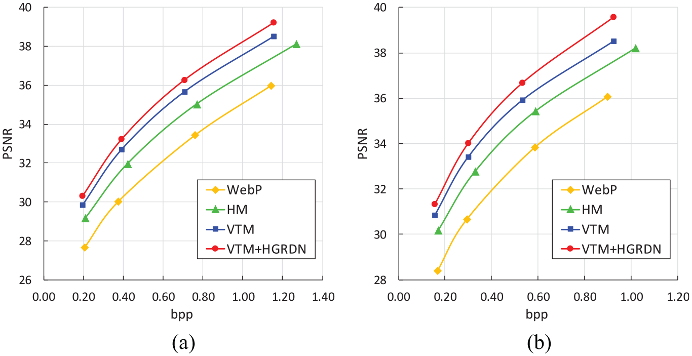
Comparisons of RD curves of the WebP, HM, VTM, and HGRDN combined with the VTM for the test datasets: (a) KODAK PhotoCD and (b) CLIC 2019 test dataset.

Table 1.

Detailed experimental results for performance evaluation of the HGRDN on the KODAK PhotoCD.

Quality level	WebP			HM			VTM			VTM + HGRDN
Quality level	bpp	PSNR (dB)	MS-SSIM	bpp	PSNR (dB)	MS-SSIM	bpp	PSNR (dB)	MS-SSIM	bpp	PSNR (dB)	MS-SSIM
Q.1	1.14	35.99	0.9855	1.27	38.12	0.9899	1.16	38.50	0.9908	1.16	39.22	0.9921
Q.2	0.76	33.43	0.9755	0.77	35.03	0.9811	0.71	35.67	0.9837	0.71	36.28	0.9858
Q.3	0.38	30.03	0.9499	0.42	31.97	0.9652	0.39	32.71	0.9702	0.39	33.23	0.9734
Q.4	0.21	27.66	0.9171	0.21	29.16	0.9375	0.19	29.84	0.9449	0.19	30.29	0.9498

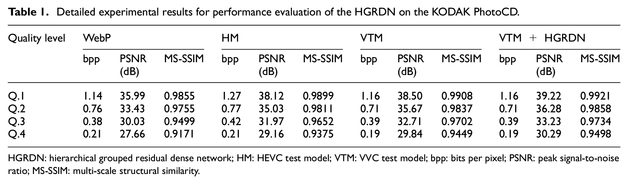
HGRDN: hierarchical grouped residual dense network; HM: HEVC test model; VTM: VVC test model; bpp: bits per pixel; PSNR: peak signal-to-noise ratio; MS-SSIM: multi-scale structural similarity.

Table 2.

Detailed experimental results for performance evaluation of the HGRDN on the CLIC 2019 test dataset.

Quality level	WebP			HM			VTM			VTM + HGRDN
Quality level	bpp	PSNR (dB)	MS-SSIM	bpp	PSNR(dB)	MS-SSIM	bpp	PSNR (dB)	MS-SSIM	bpp	PSNR (dB)	MS-SSIM
Q.1	0.90	36.06	0.9844	1.02	38.21	0.9890	0.93	38.53	0.9900	0.93	39.59	0.9916
Q.2	0.59	33.84	0.9756	0.59	35.42	0.9804	0.53	35.93	0.9828	0.53	36.69	0.9849
Q.3	0.29	30.66	0.9546	0.33	32.77	0.9675	0.30	33.41	0.9718	0.30	34.01	0.9747
Q.4	0.17	28.41	0.9284	0.17	30.19	0.9467	0.16	30.84	0.9533	0.16	31.32	0.9574

HGRDN: hierarchical grouped residual dense network; CLIC: Challenge on Learned Image Compression; HM: HEVC test model; VTM: VVC test model; bpp: bits per pixel; PSNR: peak signal-to-noise ratio; MS-SSIM: multi-scale structural similarity.

Figure 10.

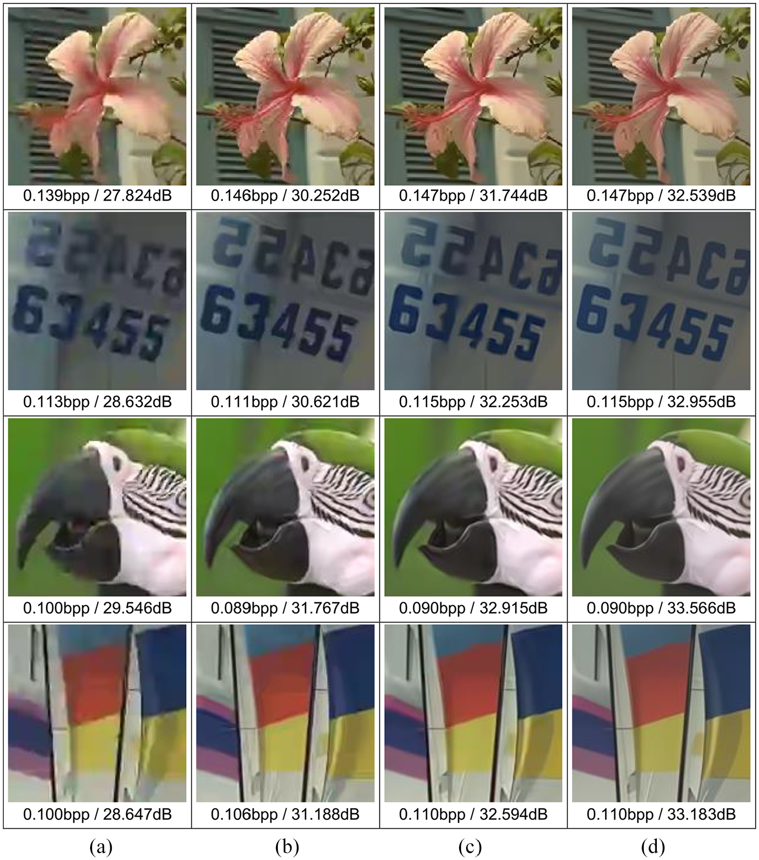
Subjective image quality of the KODAK images encoded with (a) WebP, (b) HM, (c) VTM, and (d) VTM + HGRDN.

Conclusion

In this article, HGRDN is introduced to effectively remove the compression artifacts of the VVC intra-coded images. Non-architectural aspects, which considerably affect HGRDN’s training efficiency and performance, are explored through a number of experiments. To find out an efficient HGRDN architecture, possible top-, middle-, and bottom-level HGRDN architectures are designed and they are tested in various combinations. The determined HGRDN architecture thoroughly utilizes hierarchical features in every architectural level to maximize the performance of VVC artifact reduction. From the result of the experiments to verify the RD performance, it is proved that the proposed HGRDN effectively removes the VVC artifacts over a wide bitrate range. Subsequent research of this work can be video in-loop filtering using DNN such as HGRDN. For example, one or more of the in-loop filters in VVC, deblock, sample adaptive offset (SAO), and adaptive loop filter (ALF) may be replaced with a DNN. Alternatively, a DNN can be applied as an additional in-loop filter to the existing ones. In both cases, the effect of pixel blocks restored by the DNN on inter-frame prediction should be carefully studied and harmonization with other tools should be considered.

Footnotes

Handling Editor: Partha Roy

Declaration of conflicting interests

The author(s) declared no potential conflicts of interest with respect to the research, authorship, and/or publication of this article.

Funding

The author(s) disclosed receipt of the following financial support for the research, authorship, and/or publication of this article: This work was supported by the Institute for Information and Communications Technology Promotion (IITP) grant funded by the Korea government (MSIP; 2017-0-00072, Development of Audio/Video Coding and Light Field Media Fundamental Technologies for Ultra Realistic Tera-media).

ORCID iD

Seunghyun Cho

References

Google. A new image format for the Web, https://developers.google.com/speed/webp/ (2010, accessed: 8 August 2019).

Bellard

. BPG image format, http://bellard.org/bpg/ (2014, accessed 8 August 2019).

Ascenso

Akayzi

. Report on the state-of-the-art of learning based image coding. In: Proceedings of the 83rd JPEG meeting (ISO/IEC JTC 1/SC29/WG1, document N83058), Geneva, 17–22 March 2019. Geneva: ISO.

Ascenso

Akayzi

JPEG AI image coding common test conditions. In: Proceedings of the 84th JPEG meeting (ISO/IEC JTC 1/SC29/WG1, document N84035), Brussels, 13–19 July 2019. Geneva: ISO.

Theis

Shi

Cunningham

, et al. Lossy image compression with compressive autoencoders. In: Proceedings of the 5th international conference on learning representations (ICLR), Toulon, 24–26 April 2017. La Jolla, CA: ICLR, http://arxiv.org/abs/1703.00395

Ballé

Laparra

Simoncelli

. End-to-end optimized image compression. In: Proceedings of the 5th international conference on learning representations (ICLR), Toulon, 24–26 April 2017. La Jolla, CA: ICLR, http://arxiv.org/abs/1611.01704

Ballé

Minnen

Singh

, et al. Variational image compression with a scale hyperprior. In: Proceedings of the 6th international conference on learning representations (ICLR), Vancouver, BC, Canada, 30 April–3 May 2018. La Jolla, CA: ICLR, http://arxiv.org/abs/1802.01436

Minnen

Ballé

Toderici

. Joint autoregressive and hierarchical priors for learned image compression. In: Proceedings of advances in neural information processing systems (NIPS), Montreal, QC, Canada, 2–8 May 2018. San Diego, CA: NIPS, https://arxiv.org/abs/1809.02736

Lee

Cho

Beack

S-K

. Context-adaptive entropy model for end-to-end optimized image compression. In: Proceedings of the 7th international conference on learning representations (ICLR), New Orleans, LA, 6–9 May 2019. La Jolla, CA: ICLR, https://arxiv.org/abs/1809.10452

10.

Wang

Simoncelli

Bovik

. Multiscale structural similarity for image quality assessment. In: Proceedings of the 37th Asilomar conference on signals, systems & computers (ACSSC), Pacific Grove, CA, 9–12 November 2003. New York: IEEE.

11.

Bross

Chen

Liu

. Versatile video coding (draft 6). In: Proceedings of the 15th JVET meeting (Document JVET-O2001), Gothenburg, 3–12 July 2019. Geneva: ISO.

12.

Bross

Han

W-J

Sullivan

, et al. High efficiency video coding (HEVC) text specification draft 10. In: Proceedings of the document JCTVC-L1003, Geneva, 14–23 January 2013. Geneva: ISO.

13.

Requirements. Requirements for a future video coding standard v5. In: Proceedings of the 119th MPEG meeting (ISO/IEC JTC1/SC29/WG11, document N17074), Torino, July 2017. Geneva: ISO.

14.

Chen

Kim

. Algorithm description for versatile video coding and test model 5 (VTM 5). In: Proceedings of the 14th JVET meeting (JVET-N1002), Geneva, 19–27 March 2019. Geneva: ISO.

15.

Versatile video coding reference software version 5.0 (VTM-5.0), https://vcgit.hhi.fraunhofer.de/jvet/VVCSoftware_VTM/tags/VTM-5.0/ (accessed 8 August 2019)

16.

High efficiency video coding reference software version 16.20 (HM-16.20). https://hevc.hhi.fraunhofer.de/svn/svn_HEVCSoftware/tags/HM-16.20/ (accessed 8 August 2019).

17.

Bossen

Norkin

, et al. AHG report: test model software development (AHG3). In: Proceedings of the 15th JVET meeting (JVET-O0003), Gothenburg, 3–12 July 2019. Geneva: ISO.

18.

Dong

Deng

Change Loy

, et al. Compression artifacts reduction by a deep convolutional network. In: Proceedings of IEEE international conference on computer vision (ICCV), Santiago, Chile, 7–13 December 2015, pp.576–584. New York: IEEE.

19.

Dong

Loy

, et al. Learning a deep convolutional network for image super-resolution. In: Proceedings of the European conference on computer vision (ECCV), Zurich, 6–12 September 2014, pp.184–199. Cham: Springer.

20.

Svoboda

Hradis

Barina

, et al. Compression artifacts removal using convolutional neural networks. In: Proceedings of the 24th international conference on computer graphics, visualization and computer vision, WSCG, Plzen, 30 May–3 June 2016. Plzen: WSCG, https://arxiv.org/abs/1605.00366

21.

Guo

Chao

. Building dual-domain representations for compression artifacts reduction. In: Proceedings of the European conference on computer vision (ECCV), Amsterdam, 11–14 October 2016, pp.628–644. Cham: Springer.

22.

Cavigelli

Hager

Benini

. CAS-CNN: a deep convolutional neural network for image compression artifact suppression. In: Proceedings of international joint conference on neural network (IJCNN), Anchorage, AK, 14–19 May 2017, pp.752–759. New York: IEEE.

23.

Dai

Liu

. A convolutional neural network approach for post-processing in HEVC intra coding. In: Proceedings of 23th international conference on multimedia modeling, Reykjavik, 4–6 January 2017, pp.28–39. Cham: Springer, https://arxiv.org/abs/1608.06690

24.

Soh

Park

Kim

, et al. Reduction of video compression artifacts based on deep temporal networks. IEEE Access 2018; 6: 63094–63106.

25.

Yang

Liu

, et al. Enhancing quality for HEVC compressed videos. IEEE T Circ Syst Vid 2019; 29(7): 2039–2054.

26.

Chen

Liu

, et al. Learned image restoration for VVC intra coding. In: Proceedings of the IEEE conference on computer vision and pattern recognition (CVPR) workshops, Long Beach, CA, 16–20 June 2019. New York: IEEE.

27.

Cho

Lee

Kim

, et al. Low Bit-rate image compression based on post-processing with grouped residual dense network. In: Proceedings of the IEEE conference on computer vision and pattern recognition (CVPR) workshops, Long Beach, CA, 16–20 June 2019. New York: IEEE.

28.

Kim

D-W

Chung

Jung

S-W

. GRDN: grouped residual dense network for real image denoising and GAN-based real-world noise modeling. In: Proceedings of the IEEE conference on computer vision and pattern recognition (CVPR’19), Long Beach, CA, 16–20 June 2019. New York: IEEE.

29.

Challenge on Learned Image Compression (CLIC), http://www.compression.cc/challenge/

30.

Woo

Park

Lee

J-Y

, et al. CBAM: convolutional block attention module. In: Proceedings of the European conference on computer vision (ECCV), Munich, 8–14 September 2018, pp.3–19. Cham: Springer.

31.

Huang

Liu

Weinberger

, et al. Densely connected convolutional networks. In: Proceedings of the IEEE conference on computer vision and pattern recognition (CVPR), Honolulu, HI, 21–26 July 2017, pp.4700–4708. New York: IEEE.

32.

Zhang

Tian

Kong

, et al. Residual dense network for image super-resolution. In: Proceedings of the IEEE conference on computer vision and pattern recognition (CVPR), Salt Lake City, UT, 18–22 June 2018, pp.2472–2481. New York: IEEE.

33.

Lin

T-Y

Maire

Belongie

, et al. Microsoft COCO: common objects in context. In: Proceedings of the European conference on computer vision (ECCV), Zurich, 6–12 September 2014, pp.740–755. Cham: Springer.

34.

Eastman Kodak. Kodak lossless true color image suite (PhotoCD PCD0992), 1993, http://r0k.us/graphics/kodak/

Quality enhancement of VVC intra-frame coding for multimedia services over the Internet

Abstract

Keywords

Introduction

Related works

VVC intra coding

DNN-based image quality enhancement

Proposed method

Top-level HGRDN architecture with HGRDB sub-architectures

Middle-level HGRDN architecture with GRDB sub-architectures

Bottom-level HGRDN architecture with RDB sub-architecture

Results and discussions

Implementation details and training HGRDNs

Non-architectural exploration

Architectural exploration

Experimental results

Conclusion

Footnotes

Declaration of conflicting interests

Funding

ORCID iD

References