Sage Journals: Discover world-class research

Abstract

Tensor compression algorithms play an important role in the processing of multidimensional signals. In previous work, tensor data structures are usually destroyed by vectorization operations, resulting in information loss and new noise. To this end, this article proposes a tensor compression algorithm using Tucker decomposition and dictionary dimensionality reduction, which mainly includes three parts: tensor dictionary representation, dictionary preprocessing, and dictionary update. Specifically, the tensor is respectively performed by the sparse representation and Tucker decomposition, from which one can obtain the dictionary, sparse coefficient, and core tensor. Furthermore, the sparse representation can be obtained through the relationship between sparse coefficient and core tensor. In addition, the dimensionality of the input tensor is reduced by using the concentrated dictionary learning. Finally, some experiments show that, compared with other algorithms, the proposed algorithm has obvious advantages in preserving the original data information and denoising ability.

Keywords

Tensor signal compression Tucker decomposition sparse representation dictionary learning denoising ability

Introduction

To meet the great burden in the process of transmission and storage brought by multidimensional (MD) signal processing and complete efficient extraction of signal features, more and more researchers are focusing on the tensor representation of MD signals. The study of tensor compression algorithms has become a hot research topic today.

In tensor processing, the most basic methods are canonical polyadic (CP) decomposition and Tucker decomposition. The CP decomposition serves the tensor as a sum of finite rank-one tensors.¹ Tucker decomposition decomposes a tensor into a core tensor and matrix product on each modulo.² Due to the practical requirement, many tensor processing algorithms, such as non-negative tensor decomposition,³ non-negative Tucker decomposition,⁴ and high-order singular value decomposition (HOSVD) decomposition,^5,6 have been derived by adding different constraints. To extract and fuse data features effectively, so as to realize the effective recognition and transmission of data, the researchers proposed two types of compression algorithms based on the abovementioned tensor processing methods. The one is based on the tensor decomposition, and the other is based on the sparse representation of the tensor. The following two aspects of research work will be described in detail.

On one hand, Kuang et al.⁷ proposed a tensor-based big data scalar dimensionality reduction method, in which the new data are projected into the tensor modulus expansion matrix space to achieve dimensionality reduction. In addition, the kernel-based tensor sparse dictionary learning algorithm (K-PCD) based on CP decomposition was proposed. It is an extension of the $k$ singular value decomposition (K-SVD) on tensor data.⁸ Afterward, the large scale–distributed dimensionality reduction method was developed to achieve tensor compression in the distributed computing environment.⁹ However, in this dimensionality reduction method, the high-order structure and intrinsic correlation inherent are destroyed in the original data,¹⁰ resulting in information loss or masking the redundant information and high-order dependence of original data.¹¹

On the other hand, the sparse representation of the tensor was applied to the processing of MD signals. Due to the equivalence of the tensor Tucker model and the Kronecker representation, the tensor can be defined as a representation of a given Kronecker dictionary with certain sparsity, such as multidirectional sparsity and block sparsity.¹² The corresponding Kroneker orthogonal matching pursuit (Kroneker-OMP) and N-way block OMP (N-BOMP) algorithms were also used to recover MD signals with fixed dictionaries. In addition, a dictionary learning method based on tensor factorization was proposed,¹³ and some approximate tensor algorithms were proposed based on tensor decomposition^14,15 or tensor low rank approximation.^16,17 However, in the process of tensor dictionary learning, new noise will be generated, affecting the accuracy of data,^18,19 and the determination of sparsity will bring some difficulties to tensor compression.

To solve the abovementioned problems, this article utilizes two dimensionality reduction ideas of the multilinear principal component analysis (MPCA) and the concentrated dictionary learning (CDL) to realize the tensor compression. First, the tensor is sparsely represented and Tucker decomposed to obtain the dictionary, sparse coefficient, and core tensor. Next, the results of the first step are fused to obtain a new sparse representation through the relationship between the sparse coefficient and core tensor. Furthermore, the dictionary of the second step is dimensionally reduced by the CDL algorithm to complete the dimensionality reduction of the input tensor. Finally, experimental results reveal that the proposed algorithm has significant advantages in retaining information of original data and denoising ability compared with other algorithms.

The rest of this article is organized as follows. Section “The proposed algorithm” introduces the proposed algorithm in detail. In the “Experiments” section, some experiments are examined to verify the proposed algorithm. Finally, the “Conclusion” section concludes this work.

The proposed algorithm

As depicted in Figure 1, the process of the proposed algorithm is divided into three parts. The first step is the sparse representation and Tucker decomposition of tensors. A new sparse representation is constructed in the second step. The dictionary dimensionality is reduced by using CDL algorithm in the third step. Finally, tensor compression is completed.

Figure 1.

The flow chart of the proposed algorithm.

Before describing the algorithm in detail, let us introduce the sparse representation and Tucker decomposition of the tensor, which will be useful in the sequel.

Given a tensor signal $X \in R^{I_{1} \times I_{2}, \dots, I_{N}}$ , the $n - mode$ unfolding vector of the tensor $X$ is obtained by fixing every index except the one in the mode $n$ .²⁰ $X_{n} \in R^{I_{n} \times I_{1} I_{2}, \dots, I_{n - 1} I_{n + 1} I_{N}}$ is set by converting all $n - mode$ vectors to columns of the matrix. An $n - mode$ product of the tensor with a matrix $D \in R^{J \times I_{n}}$ can be written as

Y = W \times_{n} D \in R^{I_{1} \times I_{2}, \dots, I_{n - 1} \times J \times I_{n + 1} \times I_{N}}

(1)

Note that Caiafa and Cichocki²¹ pointed out the relationship between the Kronecker model and Tucker representation. Given the $n - mode$ dictionary $D$ = { $D_{1}, D_{2}, \dots, D_{N}$ }, and $D_{n} \in R^{J_{n} \times I_{n}} (n = 1, 2, \dots, N)$ , the representation of $Y$ can be written as

Y = X \times_{1} D_{1} \times_{2} D_{2} \dots \times_{N} D_{N}

(2)

by stacking all the one-mode vectors.^22,23 After the above analysis, the sparse representation of the tensor $Y$ can be expressed as

\bar{Y} = S \times_{1} D_{1} \times_{2} D_{2} \dots \times_{N} D_{N}

(3)

where $\bar{Y}$ indicates the signal after sparseness and $S$ is the sparse coefficient tensor.

Given a tensor signal $X \in R^{I \times J \times K}$ , its Tucker decomposition is

\begin{matrix} X = Z \times_{1} A \times_{2} B \times_{3} C \\ = \sum_{p = 1}^{P} \sum_{q = 1}^{Q} \sum_{r = 1}^{R} z_{pqr} a_{p} b_{q} c_{r} \\ = [[Z; A, B, C]] \end{matrix}

(4)

where $A \in R^{I \times P}$ , $B \in R^{J \times Q}$ , and $C \in R^{K \times P}$ , and they are usually orthogonal matrices. The $Z \in R^{P \times Q \times R}$ is the core tensor.²⁴ Figure 2 displays a schematic diagram of the Tucker decomposition of a three-order tensor.

Figure 2.

Tucker decomposition of a three-order tensor.

More generally, for the $N - order$ tensor X , its Tucker decomposition is

X = Z \times_{1} A_{1} \times_{2} A_{2} \dots \times_{N} A_{N}

(5)

Tensor dictionary representation

From the above analysis, it can be found that equations (3) and (5) are similar for the same tensor. Furthermore, the sparse coefficient tensor in equation (3) is approximately equal to the core tensor in equation (5), that is, $Z \approx S$ . Here, equation (5) is transformed to obtain the following formula²⁵

Z = X \times_{1} A_{1}^{T} \times_{2} A_{2}^{T} \dots \times_{N} A_{N}^{T}

(6)

Substituting equation (6) into equation (3), we get

\bar{Y} = X \times_{1} A_{1}^{T} \times_{2} A_{2}^{T} \dots \times_{N} A_{N}^{T} \times_{1} D_{1} \times_{2} D_{2} \dots \times_{N} D_{N}

(7)

The properties of the tensor operations mentioned in Zeyde et al.²⁶ show that

When $m = n$

W \times_{m} A \times_{n} B = W \times_{n} (BA)

(8)

When $m \neq n$

W \times_{m} A \times_{n} B = W \times_{n} B \times_{m} A

(9)

Therefore, from equations (8) and (9), the objective function can be obtained

\begin{matrix} \bar{Y} = X \times_{1} A_{1}^{T} \times_{2} A_{2}^{T} \dots \times_{N} A_{N}^{T} \times_{1} D_{1} \times_{2} D_{2} \dots \times_{N} D_{N} \\ = X \times_{1} (D_{1} A_{1}^{T}) \times_{2} (D_{2} A_{2}^{T}) \dots \times_{N} (D_{N} A_{N}^{T}) \end{matrix}

(10)

Let

T_{i} = D_{i} A_{i}^{T}

(11)

Substituting equation (11) into equation (10), we get

\bar{Y} = X \times_{1} T_{1} \times_{2} T_{2} \dots \times_{N} T_{N}

(12)

where $\bar{Y}$ is the compressed signal and $X$ is the original tensor signal. One can see from the above equation that $\bar{Y}$ is the projection of the original signal $X$ with respect to the mapping matrix $T_{i}$ . In the traditional MPCA algorithm, the high-dimensional tensor achieves tensor compression by the processing of the projection matrix. In the projection matrix, the principal component retention operation is performed by the scatter matrix, and the compression is completed. Then, the high-dimensional tensor compression can be described as

W = Q \times_{1} θ_{1} \times_{2} θ_{2} \dots \times_{N} θ_{N}

(13)

where $W$ is a low-dimensional tensor signal, $Q$ is a high-dimensional tensor signal, and $θ_{i}$ is a projection matrix after dimensionality reduction. The idea of the MPCA is applied to equation (13), and the dimensionality of $T_{i}$ is reduced to achieve tensor compression and obtain a low-dimensional tensor.

Dictionary preprocessing

In the dimensionality reduction process of $T_{i}$ , the dimensionality reduction of dictionary $D$ in the mapping matrix $T_{i}$ is realized by using the idea of dimensionality reduction of dictionary in the CDL algorithm, from which some important geometric features (inner product, distance, and angle) can be preserved, the original signal can be recovered from low-dimensional data, and a dictionary pair (high-dimensional dictionary $D$ and low-dimensional dictionary $P$ ) is trained. Dictionary $D$ is used to acquire sparse representation coefficients. Dictionary $P$ is the direct dimensionality reduction sampling of $D$ . The CDL algorithm can ensure that most of the energy in $D$ is gathered by $P$ . In this way, the problem of dimensionality reduction and recovery of the signal is transformed into the training problem of the dictionary pair. The dimensionality reduction of the signal is the energy retention process from $D$ to $P$ .²⁷

The main idea of the CDL algorithm is based on the conclusions drawn in previous literature.^28–30 For the original signal $X$ and compressed signal $Y$ , the high-dimensional dictionary $D$ and the low-dimensional dictionary $P$ share a sparse representation coefficient $α$ . Then $α$ becomes a bridge between $X$ and $Y$

{\begin{matrix} X = D α + ε_{1} \\ Y = P α + ε_{2} \end{matrix}

(14)

where $ε_{1} \in R^{m} and ε_{2} \in R^{d}$ . To complete the compression, it is necessary to complete the dimensionality reduction of the dictionary $D$ to the dictionary $P$ .

To make $D$ and $P$ satisfy equation (14), $D$ needs to satisfy two conditions: (1) $D$ should make sparse coefficients of the input signal sufficiently sparse. (2) The singular value $θ = (\begin{matrix} θ_{d} & 0 \\ 0 & θ_{r} \end{matrix})$ of $D$ must be sufficiently large from $θ_{d}$ , and $θ_{r}$ must be sufficiently small not to be 0. Here, $θ_{d}$ and $θ_{r}$ are the first $d$ and the last $r$ singular values, respectively. To satisfy the above conditions, dictionary $D$ needs to be preprocessed by the process $Γ (D)$ , which can be expressed as

D^{T} D = u Λ v^{T}

(15)

where $u, v$ can be obtained by the singular value decomposition, and $Λ$ is the singular value

Λ = (\begin{matrix} Λ_{d} & 0 \\ 0 & Λ_{r} \end{matrix})

(16)

Then, the singular value is updated as

{\hat{Λ}}_{d} = \frac{Λ_{d}}{‖ Λ_{d} ‖} \cdot k \cdot t_{d}, {\hat{Λ}}_{r} = \frac{Λ_{r}}{‖ Λ_{r} ‖} \cdot k \cdot (1 - t_{d})

(17)

where $k$ is the sparsity, $t_{d}$ is the principal component threshold, and ${\hat{Λ}}_{d}$ and ${\hat{Λ}}_{r}$ are the updated singular values. The new singular value can be obtained

\hat{θ} = (\begin{matrix} \sqrt{{\hat{Λ}}_{d}} & 0 \\ 0 & \sqrt{{\hat{Λ}}_{r}} \end{matrix})

(18)

Finally, gain a new dictionary

\hat{D} = U \hat{θ} V^{T}

(19)

where $U and V$ are determined by the singular value decomposition. Thus, $\hat{D}$ is used as the input for the next dictionary update phase.

Dictionary update

In the CDL algorithm, the two-dimensional signal is used, and the dictionary can be updated by the K-SVD algorithm. However, in the high-dimensional tensor, the K-SVD algorithm cannot be used for dictionary update of high-dimensional signals. Here, the tensor-based multidimensional dictionary learning algorithm (TKSVD)³¹ is utilized to complete the dictionary update process for high-dimensional tensor signals. There are two points to be noticed in the TKSVD algorithm: (1) different from other two-dimensional signal learning methods, according to the definition of the tensor norm, the MD dictionary learning method is got

\begin{matrix} ‖ X - S \times_{1} D_{1} \dots \times_{N} D_{N} ‖_{F}^{2} \\ = ‖ X_{i} - D_{i} G_{i} C_{i} ‖_{F}^{2} \\ = ‖ X_{i} - D_{i} (G_{i} C_{i}) ‖_{F}^{2} \end{matrix}

(20)

where $C_{i} = (I_{T} \otimes D_{N} \otimes \dots \otimes D_{1})^{T}$ , $G_{i}$ indicates the atomic geometry to be removed, and $I_{T}$ represents a $T - order$ unit matrix. Obviously, it can be solved by the least squares method, and the updated value of the dictionary $D_{i}$ can be obtained

D_{i} = y_{i} {(G_{i} C_{i})}^{†}

(21)

where † represents a pseudo inverse matrix, that is, $M^{†} = M^{T} (M M^{T})^{- 1}$ . (2) After completing an iteration, the absolute error and relative error (RE) between the recoverable data and original data can be calculated under the current dictionary and sparse coefficients. The absolute error after the $i - th$ iteration is still a quantity of Frobenius norm definition

E_{G}^{i} = ‖ X - S \times_{1} D_{1} \dots \times_{N} D_{N} ‖_{F}^{2}

(22)

The $E_{G}^{i}$ is similar to the proof process of error matrix in K-SVD algorithm, in which $E_{G}^{i}$ decreases monotonously and converges. Therefore, the processing of the TKSVD algorithm improves the denoising ability of the algorithm and system stability.

The detailed algorithm flow of tensor compression is depicted in Algorithm 1. It can be seen from the algorithm flow that the proposed algorithm only contains one loop iterative process. In other words, when the dictionary is updated, only steps 5–9 are performed. Assume that there are $n$ iterations, each iteration is accompanied by $I_{N}$ cycles to update the dictionary. Then, the time complexity of the proposed algorithm is about $O (n I_{N})$ , implying that the proposed algorithm is generally lower than or equal to other algorithms in the level of time complexity, and has obvious advantages in denoising and retaining information.

Algorithm 1. Tensor compression algorithm
Require:
Train sample $X \in R^{I_{1} \times I_{2} \times \dots \times I_{n} \times T}$ , sparsity $k$ , maximum number of iterations, termination threshold $ε$ .
Ensure:
Low-dimensional tensor $\bar{Y} = X \times_{1} T_{1} \times \dots \times_{N} T_{N}$ .
1. Initialization: put the dictionary $D_{i} \in R^{I_{i} \times I_{i}} (i = 1, 2, \dots, N)$ as a Gaussian matrix and normalize the columns of each dictionary.
2. Tucker decomposition: $X = Z \times_{1} A_{1} \times_{2} A_{2} \dots \times_{N} A_{N}$ .
3. Preprocess the dictionary: $Γ (D)$
4. $n = 0$ ,
$S = X \times_{1} A_{1}^{T} \times_{2} A_{2}^{T} \dots \times_{N} A_{N}^{T}$ ,
$E = ‖ X - S \times_{1} D_{1} \dots \times_{N} D_{N} ‖_{F}^{2}$ .
5. $n - th$ dictionary update,
For $k = 1 : I_{N}$ ,
$D_{i} = X_{(i)} (G_{i} C_{i})^{†}$ ,
End.
6. Normalize dictionary $D_{i}$ .
7. Use $D_{i}$ to update $S$ .
8. After $i - th$ updates, calculate $E_{G}^{i}$ and relative errors $E_{r}$ .
9. If $E_{r} < ε$ or the number of iterations exceeds the maximum limit, terminate the loop, otherwise continue to steps 5–9.
10. Calculate $U_{d}$ :
$D = U Θ V^{T} = [\begin{matrix} U_{d} & U_{r} \end{matrix}] [\begin{matrix} Θ_{d} & 0 \\ 0 & Θ_{r} \end{matrix}] {[\begin{matrix} V_{d} & V_{r} \end{matrix}]}^{T}$ .
11. The low-dimensional dictionary can be obtained: $P = U_{d}^{T} D$ .
12. The low-dimensional projection matrix can be obtained: $T_{i} = P_{i} A_{i}^{T}$ .

Experiments

In this section, the RE is used to test the information retention ability of the proposed algorithm. In this regard, it will be compared with the principal component analysis (PCA), maximum noise fraction (MNF) algorithm, and MPCA. In addition, signal-to-noise ratio (SNR), peak signal-to-noise ratio (PSNR), and structural similarity index measurement (SSIM) are applied to test the denoising ability of the proposed algorithm. Here, it will be compared with PCA, the binary wavelet threshold shrinkage (PCA-Bish), and MPCA.

Reconstruction performance analysis

The dataset of the hyperspectral image library published by the Computer Vision Laboratory of the Department of Computer Science of Columbia University is applied to test the ability of retaining the original data information. The RE is used to describe the closeness of the reconstructed tensor to the original tensor, that is

P_{e} = \frac{{‖ X - X' ‖}^{2}}{{‖ X ‖}^{2}}

(23)

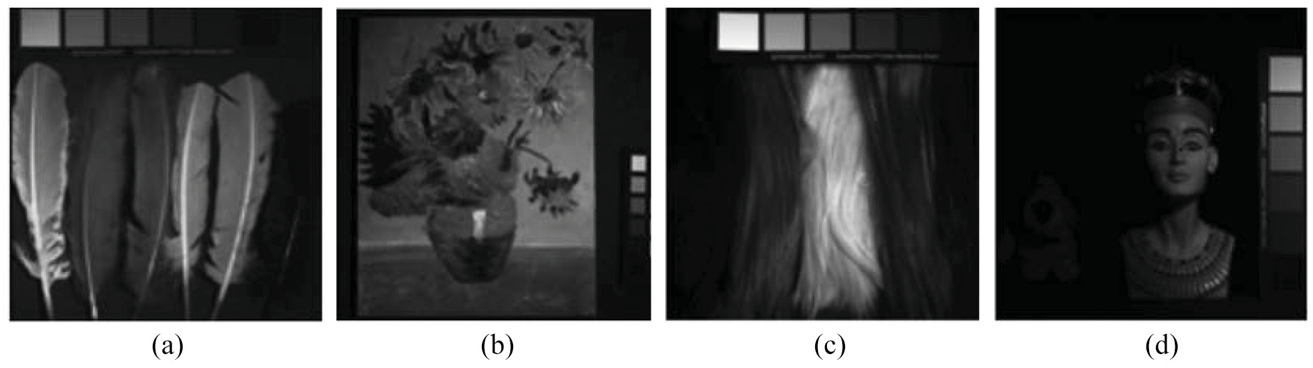
Obviously, the reconstructed tensor is closer to the original tensor with a smaller $P_{e}$ . Ideally, if the reconstructed tensor is exactly the same as the original tensor, then $P_{e} = 0$ .

Here, the spatial size of each hyperspectral image is $512 \times 512$ pixels, and the sensor can continuously image at a spectral resolution of $10 nm$ in the wavelength range of $400$ to $700 nm$ , so each hyperspectral image contains 31 spectral channels. Thus, the original third-order observation tensor expressed by the tensor is $512 \times 512 \times 31$ , as shown in Figure 3.

Figure 3.

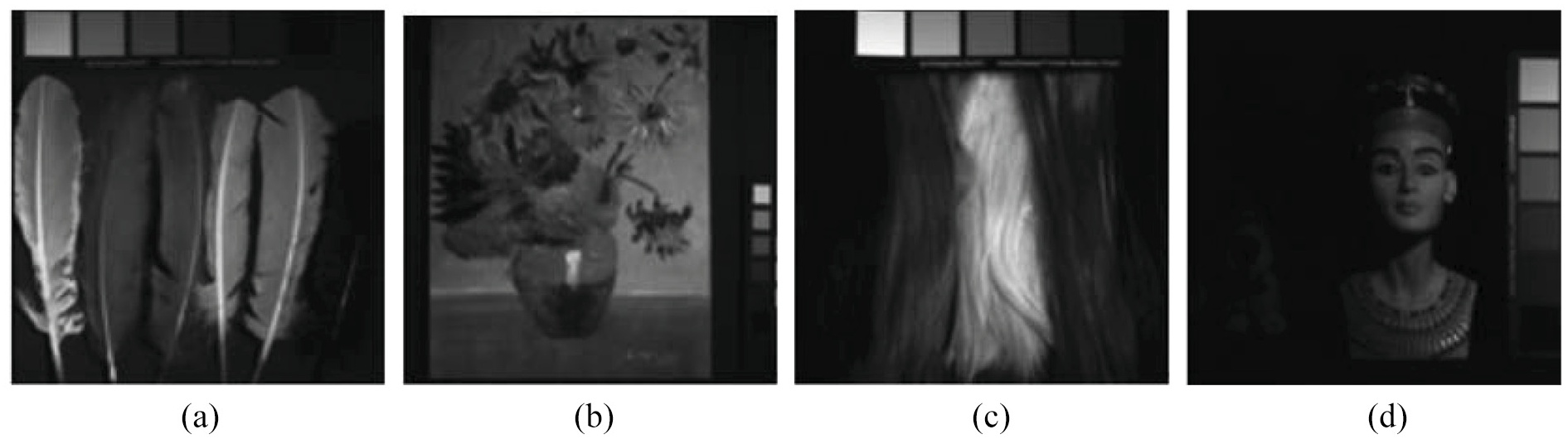
The original image: (a) feather, (b) painting, (c) hair, and (d) statue.

To test the performance of algorithm reconstruction, the hyperspectral image is compressed by the proposed algorithm according to the compression rate (CR) of 0.04, 0.08, 0.14, 0.21, and 0.27, respectively. Under the same CR, a comparison of PCA, MNF, and MPCA, RE in the 31st spectral channel is given (see Figure 4).

Figure 4.

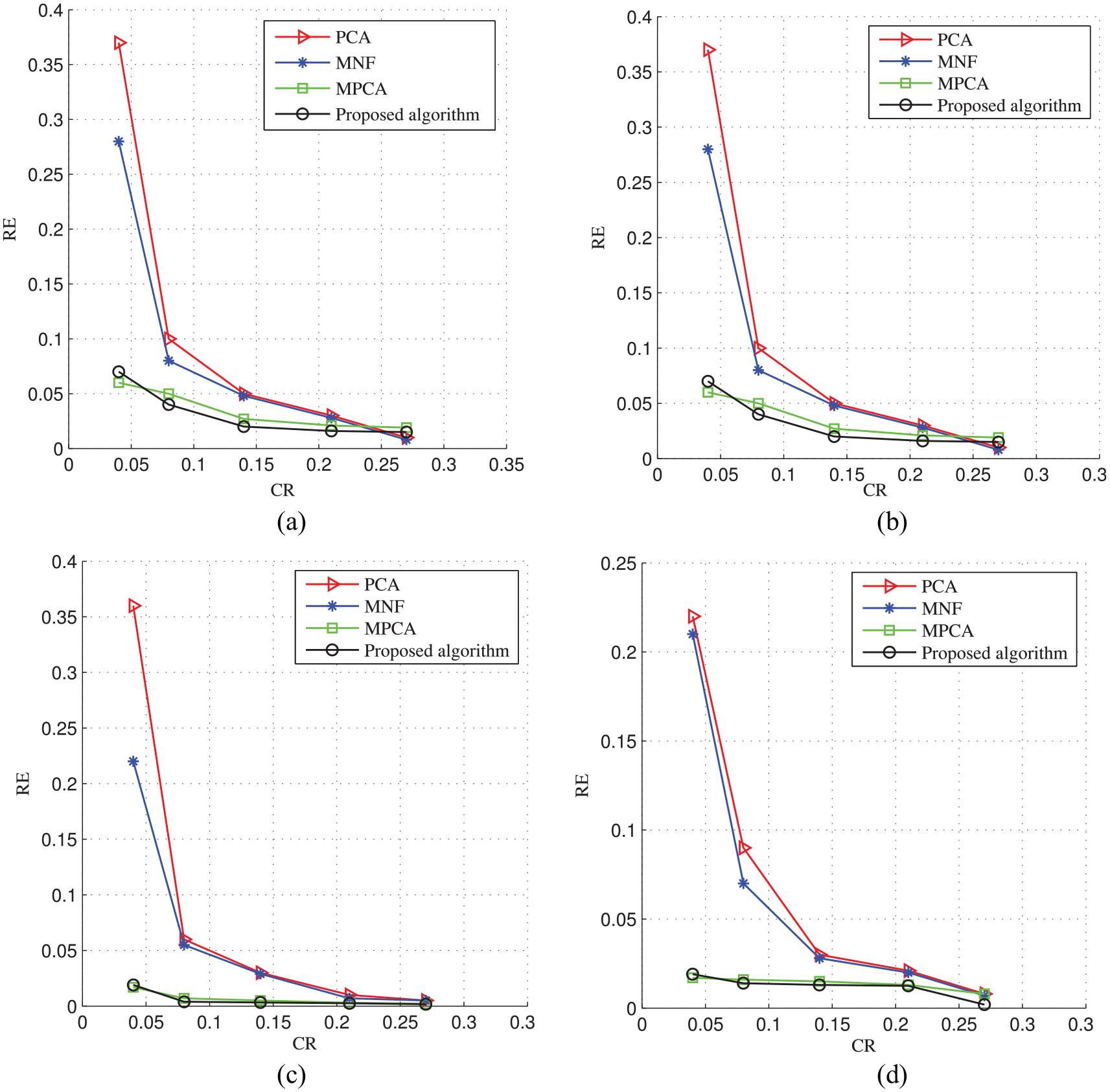
RE of hyperspectral images reconstruction under different CR: (a) feather, (b) painting, (c) hair, and (d) statue.

In the curves of Figure 4(a)–(d), the closer to the lower left of the figure, the better the performance of all algorithms. It can be seen that in the compression and reconstruction experiments of hyperspectral images, the RE of the proposed algorithm is lower than PCA and MNF under the same CR. Especially when the CR is extremely low, the RE of the proposed algorithm is slightly higher than that of the MPCA algorithm. But when the CR increases, the RE of the proposed algorithm is higher than that of the MPCA algorithm, so the overall reconstruction performance is better than the MPCA algorithm.

To verify the practicability, the CR is set to 0.01, and the original image of the 31st spectral channel and the reconstructed image of the proposed algorithm are shown in Figures 5 and 6, respectively. The RE of the reconstruction of the four groups of hyperspectral images are 0.0251, 0.0239, 0.0211, and 0.0195, respectively. Obviously, for the image hair and the statue with simple texture, the RE of reconstruction can be controlled within 0.03. Therefore, the proposed algorithm has a good practical value.

Figure 5.

Original images (spectral channel 31): (a) feather, (b) painting, (c) hair, and (d) statue.

Figure 6.

Reconstructed images (spectral channel 31): (a) feather, (b) painting, (c) hair, and (d) statue.

Robust analysis

The spectral data “splib06a” collected by the American Bureau of Geological Survey’s Digital Spectrum Laboratory using the AVIRIS (airborne visible/infrared imaging spectrometer) sensor Indian Pines³² are utilized as a dataset to test the denoising ability of the proposed algorithm.

Here, the noise is the white Gaussian noise. To verify the effectiveness of the proposed algorithm in denoising, it is compared with the following two denoising algorithms: (1) PCA denoising algorithm (abbreviated as PCA algorithm)³³ and (2) denoising algorithm combined with PCA and 2D PCA-Bish algorithm.³⁴

Figures 7 and 8 show two bands of randomly selected data from the simulated data Indian Pines with noise ( $σ = 20$ ). It can be clearly seen that the proposed algorithm can better remove the noise influence and retain the details of the original image as much as possible.

Figure 7.

Compression performance of different algorithms (spectral channel 25): (a) original image, (b) noisy image, (c) PCA, (d) PCA-Bish, and (e) proposed algorithm.

Figure 8.

Compression performance of different algorithms (spectral channel 35): (a) original image, (b) noisy image, (c) PCA, (d) PCA-Bish, and (e) proposed algorithm.

It can be seen that although the data amount of the image is greatly compressed, from the visual effect, the difference between the reconstructed image and the original image is not obvious. Thus, in addition to visual effects, SNR, PSNR, and SSIM are used to compare the performance of different methods, and they are defined as

SNR = 10 \lg \frac{\sum_{i, j, p} X {(i, j)}^{2}}{\sum_{i, j} {(\bar{X} (i, j) - X (i, j))}^{2}}

(24)

PSNR = 10 \lg \frac{255^{2}}{\sum_{i, j} \frac{{(\bar{X} (i, j) - X (i, j))}^{2}}{M \times N}}

(25)

SSIM = \frac{(2 u_{X} u_{\bar{X}} + C_{1}) (2 σ_{X} σ_{\bar{X}} + C_{2})}{(u_{X}^{2} + u_{\bar{X}}^{2} + C_{1}) (σ_{X}^{2} + σ_{\bar{X}}^{2} + C_{2})}

(26)

where $i = 1, 2, \dots, M$ , $j = 1, 2, \dots, N$ , $X$ represents no noise image data in each spectral channel, $\bar{X}$ represents noisy data or denoised data, $u_{X}$ represents the average value of the image, $X$ is the gray mean, and $σ_{X}$ represents the standard deviation (Std) of the gray of the image $X$ , and $C_{1} = (255 K_{1})^{2}$ , $C_{2} = (255 K_{2})^{2}$ , $K_{1} = K_{2} = 0.01$ .

The Indian Pines is processed by PCA, PCA-Bish, and the proposed algorithm, respectively. And SNR, PSNR, and SSIM are used to judge the robustness of the proposed algorithm.

It can be seen from the mean and Std in Table 1 that under the three kinds of noise standard deviation, the proposed algorithm has less noise than the other two algorithms, and the effect is more obvious under the condition of higher noise.

Table 1.

Comparison of denoising performance of three denoising methods (SNR/dB).

Evaluation standard	$σ$	Noisy image		PCA		PCA-Bish		Proposed algorithm
Evaluation standard	$σ$	Mean	Std	Mean	Std	Mean	Std	Mean	Std
SNR/dB	10	37.5281	0.6230	75.0122	1.5981	75.0213	1.4722	77.64227	1.2987
	15	27.9534	0.7623	65.9984	0.8701	66.9935	0.8003	72.5671	0.7534
	20	21.1321	1.2560	62.0037	0.1445	62.0145	0.9660	74.3575	0.0923

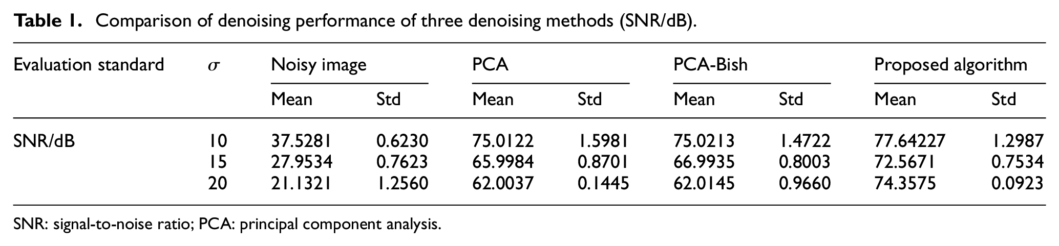
SNR: signal-to-noise ratio; PCA: principal component analysis.

Table 2 displays that under the three kinds of noise standard deviation conditions, PCA and PCA-Bish compression reconstructed image quality are similar, but the image quality processed by PCA is higher than PCA-Bish image quality when the noise is larger. Compared with the proposed algorithm, PCA has lower reconstructed image quality. Therefore, under noise conditions, the performance of the proposed algorithm is better than PCA and PCA-Bish.

Table 2.

Comparison of denoising performance of three denoising methods (PSNR/dB).

Evaluation standard	$σ$	Noisy image		PCA		PCA-Bish		Proposed algorithm
Evaluation standard	$σ$	Mean	Std	Mean	Std	Mean	Std	Mean	Std
PSNR/dB	10	18.2103	0.0201	37.9587	1.6002	37.9765	1.4961	38.0104	0.7901
	15	15.9937	0.0190	37.2101	0.9930	37.0531	0.9601	38.9890	0.7015
	20	15.5638	0.0401	36.3402	0.9402	36.0258	0.8535	38.2531	0.6231

PSNR: peak signal-to-noise ratio; PCA: principal component analysis.

Table 3 illustrates the compression performance by using SSIM. It can be seen that the SSIM values of the three algorithms are different in three cases. But considering SSIM and Std, the proposed algorithm is obviously higher than other two algorithms, and the reconstructed image is more similar to the original image. In general, due to the large number of hyperspectral image bands, the visual effect evaluation of a certain band image is insufficient to illustrate the effectiveness of the proposed algorithm. For this purpose, data analysis of all bands is required.

Table 3.

Comparison of denoising performance of three denoising methods (SSIM).

Evaluation standard	$σ$	Noisy image		PCA		PCA-Bish		Proposed algorithm
Evaluation standard	$σ$	Mean	Std	Mean	Std	Mean	Std	Mean	Std
SSIM	10	0.2139	0.0145	0.9627	0.0633	0.9649	0.0603	0.9661	0.0401
	15	0.1530	0.0142	0.9601	0.0701	0.9604	0.0584	0.9772	0.0530
	20	0.1244	0.0211	0.9601	0.0637	0.9621	0.0542	0.9635	0.0483

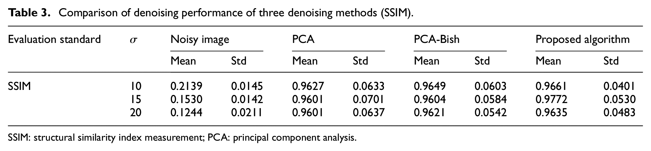
SSIM: structural similarity index measurement; PCA: principal component analysis.

By observing the data in Tables 1 –3, it can be seen that the trends of SNR, PSNR, and SSIM are basically the same. The denoising effects of the three methods are also analyzed: (1) they have no obvious advantage when the noise standard deviation is very low. This is mainly because the noisy image group generated by PCA conversion retains most of the image information when the noise is very small. The three methods except PCA will cause the loss of image detail information in denoising, and the PCA method directly uses the principal component image, so there is no such problem. (2) When the standard deviation of noise gradually increases, the advantage of the proposed algorithm becomes more obvious.

Conclusion

In this article, to solve the problems of information loss and new noise in previous work, a tensor compression algorithm using Tucker decomposition and dictionary dimensionality reduction has been proposed. The sparse coefficient and core tensor have been used to relate the sparse representation of the tensor with the Tucker decomposition. In the new sparse representation, the dimensionality reduction of the dictionary has been applied to the dimensionality reduction of the mapping matrix, and the tensor compression has been implemented. Finally, some experiments show that compared with other algorithms, the proposed algorithm can better preserve the original data information, and in the noise environment, the denoising ability of the proposed algorithm is stronger and the system is more stable.

In addition, it has to be mentioned that the approximate relationship between the sparse coefficients and core tensors plays an important role in the proposed algorithm. In the approximation process, there must be a certain approximation error. Therefore, how to reduce the error in the process is a problem worthy of study in the next research work. Meanwhile, deep learning has been widely used in many fields such as sentiment analysis^35,36 and automatic modulation classification;³⁷ thus, how to effectively apply deep learning to the field of tensor signal compression may give rise to a research field of interest.

Footnotes

Acknowledgements

The authors are grateful to the anonymous reviewers and the editor for their valuable comments and suggestions.

Handling Editor: Hongxiang Li

Declaration of conflicting interests

The author(s) declared no potential conflicts of interest with respect to the research, authorship, and/or publication of this article.

Funding

The author(s) disclosed receipt of the following financial support for the research, authorship, and/or publication of this article: This work is supported by the Natural Science Foundation of China (Grant Nos. 61702066 and 61903056), Major Project of Science and Technology Research Program of Chongqing Education Commission of China (Grant No. KJZD-M201900601), Chongqing Research Program of Basic Research and Frontier Technology (Grant Nos. cstc2017jcyjAX0256, cstc2019jcyj-msxmX0681, and cstc2018jcyjAX0154), and Project Supported by Chongqing Municipal Key Laboratory of Institutions of Higher Education (Grant No. cqupt-mct-201901).

ORCID iDs

Chenquan Gan

Zufan Zhang

References

Veganzones

Cohen

Farias

, et al. Nonnegative tensor CP decomposition of hyperspectral data. IEEE T Geosci Remote 2016; 54(5): 2577–2588.

Wang

Bai

, et al. Hyperspectral image compression based on lapped transform and Tucker decomposition. Signal Process: Image 2015; 36: 63–69.

Chi

Kolda

. On tensors, sparsity, and nonnegative factorizations. SIAM J Matrix Anal A 2012; 33(4): 1272–1299.

Zhou

Cichocki

Zhao

, et al. Efficient nonnegative Tucker decompositions: algorithms and uniqueness. IEEE T Image Process 2015; 24(12): 4990–5003.

Katkovnik

Egiazarian

. Sparse phase imaging based on complex domain nonlocal BM3D techniques. Digit Signal Process 2017; 63: 72–85.

Chen

Wei

, et al. An adaptive weighted HOSVD denoising method. In: 2017 4th international conference on information science and control engineering (ICISCE), Changsha, China, 21–23 July 2017, pp.145–149. New York: IEEE.

Kuang

Hao

Yang

, et al. A tensor-based approach for big data representation and dimensionality reduction. IEEE T Emerg Top Comput 2014; 2(3): 280–291.

Duan

Wang

Liu

, et al. K-CPD: learning of overcomplete dictionaries for tensor sparse coding. In: Proceedings of the 21st international conference on pattern recognition, Tsukuba, Japan, 11–15 November 2012, pp.493–496. New York: IEEE.

Kuang

Yang

Wang

, et al. A tensor-based big data model for QoS improvement in software defined networks. IEEE Network 2016; 30(1): 30–35.

10.

Chen

Hus

Liao

HYM

. Simultaneous tensor decomposition and completion using factor priors. IEEE T Pattern Anal 2014; 36(3): 577–591.

11.

Xie

Peng

, et al. Semi-tensor compressed sensing. Digit Signal Process 2016; 58: 85–92.

12.

Caiafa

Cichocki

. Computing sparse representations of multidimensional signals using Kronecker bases. Neural Comput 2013; 25(1): 186–220.

13.

Zubair

Wang

. Tensor dictionary learning with sparse Tucker decomposition. In: 2013 18th international conference on digital signal processing (DSP), Fira, 1–3 July 2013, pp.1–6. New York: IEEE.

14.

Nguyen

Abed-Meraim

Linh-Trung

. Second-order optimization based adaptive PARAFAC decomposition of three-way tensors. Digit Signal Process 2017; 63: 100–111.

15.

Sidiropoulos

Lathauwer

De Fu

, et al. Tensor decomposition for signal processing and machine learning. IEEE T Signal Proces 2017; 65: 3551–3582.

16.

Zhou

Cichocki

Xie

. Fast nonnegative matrix/tensor factorization based on low-rank approximation. IEEE T Signal Proces 2012; 60(6): 2928–2940.

17.

Rajwade

Rangarajan

Banerjee

. Image denoising using the higher order singular value decomposition. IEEE T Pattern Anal 2013; 35(4): 849–862.

18.

Said

Hadjidj

Melkemi

, et al. Multispectral image denoising with optimized vector non-local mean filter. Digit Signal Process 2016; 58: 115–126.

19.

Dai

Xiong

. Compressive tensor sampling with structured sparsity. In: 2016 data compression conference (DCC), Snowbird, UT, 30 March–1 April 2016, pp.181–190. New York: IEEE.

20.

Kolda

Bader

. Tensor decompositions and applications. SIAM Rev 2009; 51(3): 455–500.

21.

Caiafa

Cichocki

. Block sparse representations of tensors using Kronecker bases. In: 2012 IEEE international conference on acoustics, speech and signal processing (ICASSP), Kyoto, Japan, 25–30 March 2012, pp.2709–2712. New York: IEEE.

22.

Arguello

Rueda

, et al. Higher-order computational model for coded aperture spectral imaging. Appl Optics 2013; 52(10): 12–21.

23.

Fowler

. Reconstruction from random projections of hyperspectral imagery with spectral and spatial partitioning. IEEE J Sel Top Appl 2013; 6(2): 466–472.

24.

Yang

Zhang

Wang

, et al. A multi-affine model for tensor decomposition. In: 2011 IEEE international conference on computer vision workshops (ICCV Workshops), Barcelona, 6–13 November 2011, pp.1348–1355. New York: IEEE.

25.

Yuan

Zhao

Cao

. High-order tensor completion for data recovery via sparse tensor-train optimization. In: 2018 IEEE international conference on acoustics, speech and signal processing (ICASSP), Calgary, AB, Canada, 15–20 April 2018, pp.1258–1262. New York: IEEE.

26.

Zeyde

Elad

Protter

. On single image scale up using sparse representations. In: Proceedings of the 7th international conference on curves and surfaces, Avignon, 24–30 June 2010, pp.711–730. Berlin: Springer.

27.

Yang

Wang

Lin

, et al. Coupled dictionary training for image super-resolution. IEEE T Image Process 2012; 21(8): 3467–3478.

28.

Yang

Wright

Huang

, et al. Image super resolution via sparse representation. IEEE T Image Process 2010; 19(11): 2861–2873.

29.

Adler

Hel-Or

Elad

. A shrinkage learning approach for single image super-resolution with overcomplete representations. In: Proceedings of the 11th European conference on computer vision, Crete, 5–11 September 2010, pp.622–635. Berlin: Springer.

30.

Singh

Yamaguch

. Model-based six-component scattering matrix power decomposition. IEEE T Geosci Remote 2018; 56(10): 5687–5704.

31.

Roemer

Galdo

Haardt

. Tensor-based algorithms for learning multidimensional separable dictionaries. In: 2014 IEEE international conference on acoustics, speech and signal processing (ICASSP), Florence, 4–9 May 2014, pp.3991–3995. New York: IEEE.

32.

Zhu

Yao

Bai

. Scene text detection and recognition: recent advances and future trends. Front Comput Sci 2016; 10(1): 19–36.

33.

Stephan

Hibbitts

Hoffmann

, et al. Reduction of instrument-dependent noise in hyperspectral image data using the principal component analysis: applications to Galileo NIMS data. Planet Space Sci 2008; 56(4): 406–419.

34.

Chen

Qian

. Denoising of hyperspectral imagery using principal component analysis and wavelet shrinkage. IEEE T Geosci Remote 2011; 49(3): 973–980.

35.

Zhang

Zou

Gan

. Textual sentiment analysis via three different attention convolutional neural network and cross-modality consistent regression. Neurocomputing 2018; 275: 1407–1415.

36.

Gan

Wang

Zhang

, et al. Sparse attention based separable dilated convolutional neural network for target entities sentiment analysis. Knowl-Based Syst 2020; 188: 1–10.

37.

Zhang

Wang

Gan

, et al. Automatic modulation classification using convolutional neural network with features fusion of SPWVD and BJD. IEEE T Signal Inf Process Over Netw 2019; 5(3): 469–478.

A tensor compression algorithm using Tucker decomposition and dictionary dimensionality reduction

Abstract

Keywords

Introduction

The proposed algorithm

Tensor dictionary representation

Dictionary preprocessing

Dictionary update

Experiments

Reconstruction performance analysis

Robust analysis

Conclusion

Footnotes

Acknowledgements

Declaration of conflicting interests

Funding

ORCID iDs

References