
Abstract
This article suggested two methods to compensate for the temperature drift of the micro-electro-mechanical system gyroscopes, which are support vector machine method and C-means support vector machine. The output of X axis which was ranged from −40°C to 60°C based on the micro-electro-mechanical system gyroscope is reduced and analyzed in this article. The results showed the correctness of the two methods. The final results indicate that when the temperature is ranged from −40°C to 60°C, the factor of B is reduced from 0.424
Keywords
Introduction
The micro-electro-mechanical system (MEMS) gyroscope is an inertial sensor based on the technology of MEMS, which is used to sense the rotation rate of the carrier. The outstanding characteristics of the MEMS gyroscope are small size, light weight, low power consumption, and batch production. Low-precision MEMS gyroscope products have been very popular in the civil market and are widely used in consumer electronics and automotive fields. At the same time, the MEMS gyroscope is also widely used in the fields of attitude control and vehicle-borne satellite antenna. Most authors pay attention to improve the performance of MEMS gyroscopes. However, two main methods are used to improve their performance.1,2
On one hand, one way is using hardware methods to reduce the temperature drift of the MEMS gyroscope. Therefore, most hardware methods have been suggested which contain structure and circuit. For instance, Cao et al. 3 proposed that a bandwidth expansion method for dual-mass MEMS gyroscopes based on the pole-zero temperature compensation method. Cao et al. 4 also proposed a sense mode closed-loop method for dual-mass MEMS gyroscopes based on the bi-pole temperature compensation method, and the experiment results show the bias temperature coefficient is decreased to 9.534°/h/°C and 5.991°/h/°C, respectively, based on sense open-loop and closed-loop circuits. Ou et al. 5 investigated a new stress-released structure to improve the performance of temperature stability of MEMS gyroscope. Li et al. 6 proposed a new method named frequency mismatch control to improve the temperature stability sensitivity for MEMS gyroscope. The results show that the scale factor temperature coefficient reduces from 1300 to 282.12 ppm/°C. Cao et al. 7 proposed a new structure, which is a vibration ring gyroscope with a double U-beam and designed using a combination of mathematical analysis and the finite-element method. This new structure can easily improve performance. Although hardware methods have effectively improved the performance of MEMS gyroscopes under different temperature, these methods spend more time and amount of work.
On the other hand, the other way is to establish the mathematical model is to reduce temperature drift that is reported as software compensation. Fu et al.
8
introduced the principle of MEMS gyroscope and the influence of MEMS gyroscope based on the temperature characteristic. Cao et al.
9
proposed a method which called radial basis function neural network (RBF NN) to compensate the temperature energy influence. The results indicate that, after RBF NN-GA-KF method compensation, the bias instability of Gyros X, Y, and Z improves from
In this article, for the sake of improving the performance, a temperature drift model is established, and some methods are suggested to compensate for temperature drift. The algorithm of SVMs which is first used in temperature compensation of MEMS gyroscope is suggested to analyze and reduce the drift. Instead of a single algorithm, a novel improved SVMs algorithm is also suggested to reduce the drift. The Allan variance is suggested to compare the performance of compensation and improve the availability and practicability of the suggest methods.
Model of MEMS gyroscope and temperature
Structure model of MEMS gyroscope
As it is shown in Figure 1, the structure of this MEMS gyroscope can be divided into two modes: drive mode and sense mode, which can be described as a spring-mass-damping second-order system. It can be shown that the drive mode has 1 degree of freedom (DOF) along the X axis, and the sense mode also has 1 DOF along the Y axis. Each axis has two sections, which are stiffness


where

The structure of drive and sense mode.
Therefore, the natural frequency and the damping ratio of the drive mode should be described as

By solving equation (1), the displacement of the MEMS gyroscope in the drive direction can be described as

where the phase and amplitude should be determined as


When the MEMS gyroscope gets an angular velocity

where
So, the equation of motion in sense mode is given as

where the natural frequency and the damping ratio of the sense mode should be described as

By solving equation (1), the displacement of the MEMS gyroscope in the sense direction can be described as

where the phase and amplitude should be determined as


The temperature model and drift of MEMS gyroscope
Temperature is one of the most significant factors that affects the performance of the MEMS gyroscope. There are two main factors that are to be considered: the size of the structure and the material of the elastic modulus when the temperature is changed. Among the two factors, the size of the structure has less influence on the performance of gyroscopes and the influence of the material of the elastic modulus should be mainly discussed.
The stiffness of the MEMS gyroscope system will be changed when the material of the elastic modulus is changed and the resonant frequency also changes with the stiffness of the system. Therefore, the change of temperature will lead to the drift of resonant frequency. Obviously, elastic modulus varies linearly with the temperature as shown in the following equation

where

where

So, we can see from these equations that temperature is one of the most significant factors which affects the performance of the MEMS gyroscope.
The experiment of temperature
The MEMS gyroscope is placed at the inside of a temperature-controlled oven for the sake of outputting the signal and not being affected by temperature variations of environment; the ranges of temperature and the temperature rate are set from −40°C to 60°C and 1°C/min, respectively. First, the initial temperature should be set as 60°C and placed in the temperature for an hour to ensure that the structural temperature is stable at 60°C. Then, the temperature is decreased at a rate of −1°C/min to −40°C and that temperature is also maintained for an hour to ensure that the structural temperature is of −40°C. The temperature-controlled oven should be observed at every 10°C for an hour to collect the data and be ensured that the structural temperature has a good stability and equal to oven temperature. The environment and steps are shown in Figure 2.
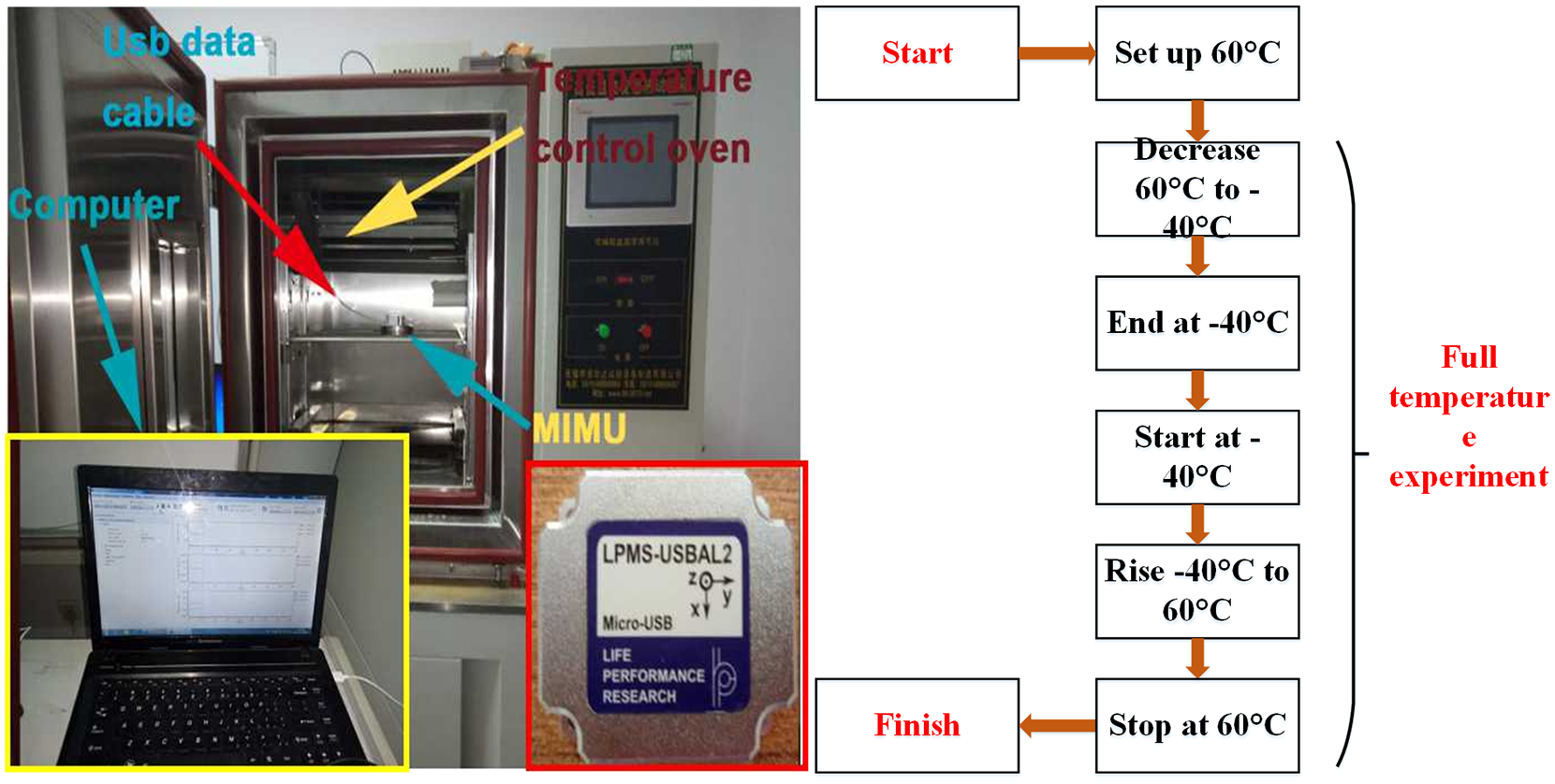
The equipment of temperature experiment.
As for the test, the original output of an axis which described the output data reduce from 60°C to −40°C and rise from −40°C to 60°C is shown in Figure 3.

The original output data of MEMS gyroscope: (a)
The model of temperature and algorithms
The drift model of temperature based on algorithms
A novel temperature drift model is established in this article: temperature and temperature variation rate. These two factors could reflect the performance perfectly, therefore,

where

Algorithm of SVMs
SVMs 16 are based on the theory of statistical learning theory (SLT). SLT has several characteristics such as intuitive geometric explanations and perfect mathematical forms. Since Vapnik put forward the concept of SVM in the 1990s, the basic framework of algorithmic and theoretical concepts has been completely determined, which is based on many kinds of SVMs.
With the majority of data samples based on SVM, we can describe that the linear separable samples are considered as two classes, which are

and its standard form can be constrained by the expression of above equation

Figure 4 shows the classification of a sample hyperplane. We can focus on that the distance from the point of the data sample to the hyperplane is described as the equation
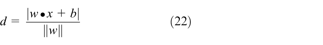

The classification of sample hyperplane.
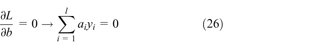
This distance is called the classifications distance, and the maximum distance classification is required. In order for the maximum classification interval to be equivalent to the minimum of values of


where

where the Lagrange factor is

We can also express the question of dual optimization by equations (27)–(29)

where

where
As for non-linear data samples, the non-linear transformation can be transformed into another linear question in high-dimensional space to solve, which needs to be achieved by the kernel function such as

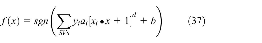
and the function of classification becomes

In conclusion, these are SVMs. The kernel function is one of the most significant factors in the algorithm of SVM. The present kernel function makes the function solution bypass the eigenspace and get directly in the input space which avoids computational jealousy of non-linear mappings. There are some general kernel functions such as linear kernel function (LKF), polynomial kernel function (PKF), sigmoid kernel function (SKF), radial basis kernel function (RBKF), and spline kernel function (SPKF) which are described as follows
LKF

PKF

SKF

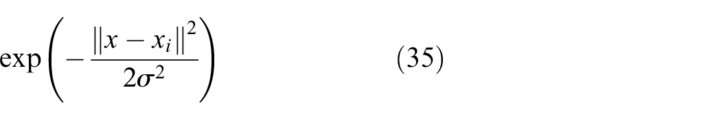
RBKF
SPKF

As is shown on these equations, LKF is a typical global kernel function that can be regarded as classifying the linearly separable data sets. PKF is an extensive applied non-linear mapping function, and the approaching capability of it is determined by the order of the polynomial. PKF is a d-order polynomial classifier which can be described as the above function
SKF actually includes a multi-layer perceptron network with a hidden layer, but the weight and the amount of hidden layer nodes are automatically determined by the algorithm, unlike the traditional perceptron network, which is determined by human experience. RBKF is the most extensive applied localized kernel function and strong in local regression. The smaller the value of
Improved algorithm of SVMs
An improved SVM algorithm which is based on fuzzy C-means clustering is suggested to compensate for temperature drift more effectively. The SVM algorithm based on fuzzy C-means clustering includes three main processes which are shown in Figure 5. The processes are to use the fuzzy C-means clustering to preprocess the data of the learning sample. The second process is to describe the application of different classes SVM algorithm which is generated clustering by different classifications. The third process is to calculate the distance from the sample to each clustering center. Finally, the results of the whole system output for each calculation results of SVM algorithm. The steps of C-means support vector machine (C-SVM) method are shown in Figure 5.

The steps of C-SVM algorithm.
The steps of C-SVM method is as follows:
Step1: Judging whether pre-clustering is necessary according to the size of learning sample data. As the number of clusters is larger than the set value, the number of clusters is calculated and the fuzzy C-means clustering is performed.
Step 2: As for each sample, find out the maximum membership degree of each cluster center and classify it into corresponding classes.
Step 3: After the clustering is completed, the number of samples contained in each class is calculated. And if the number is less than the corresponding value, the relevant class centers and the number of redundant classes will be eliminated. The samples are clustered again according to the new cluster number.
Step 4: Different SVMs are used to learn different classes.
Step 5: A fuzzy classifier is constructed to get the output of SVM. The input for each membership degree of sub-SVM is determined. According to the membership degree, the output of each sub-SVM model is synthesized and the final output is obtained
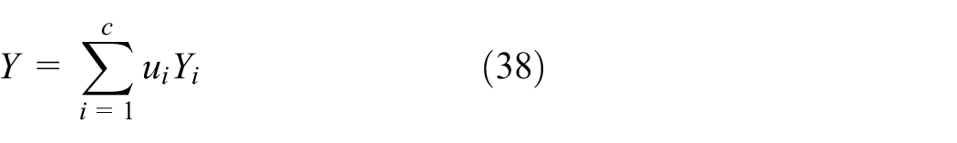
where

where
Computation complexity of SVM and C-SVM
In order to compare the computation complexity of SVM and C-SVM, computation time and space complexity is provided in this article. In order to analyze, we assume that the time spent for all operators is the same and the computation complexity concerns only performance and running hardware. After running the algorithms based on MATLAB, the results are shown in Table 1.
The results of computation time and space complexity based on SVM and C-SVM.
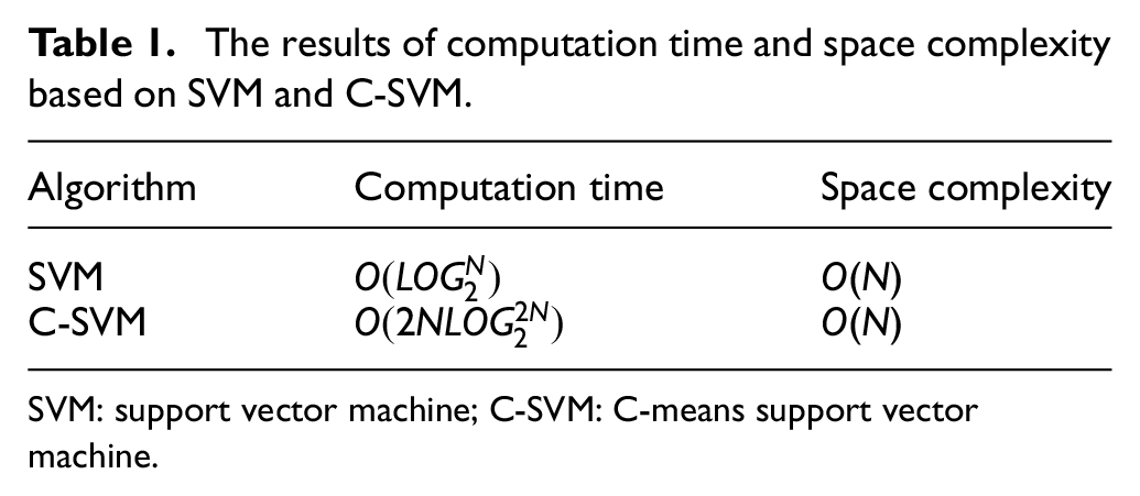
SVM: support vector machine; C-SVM: C-means support vector machine.
Verification and analysis
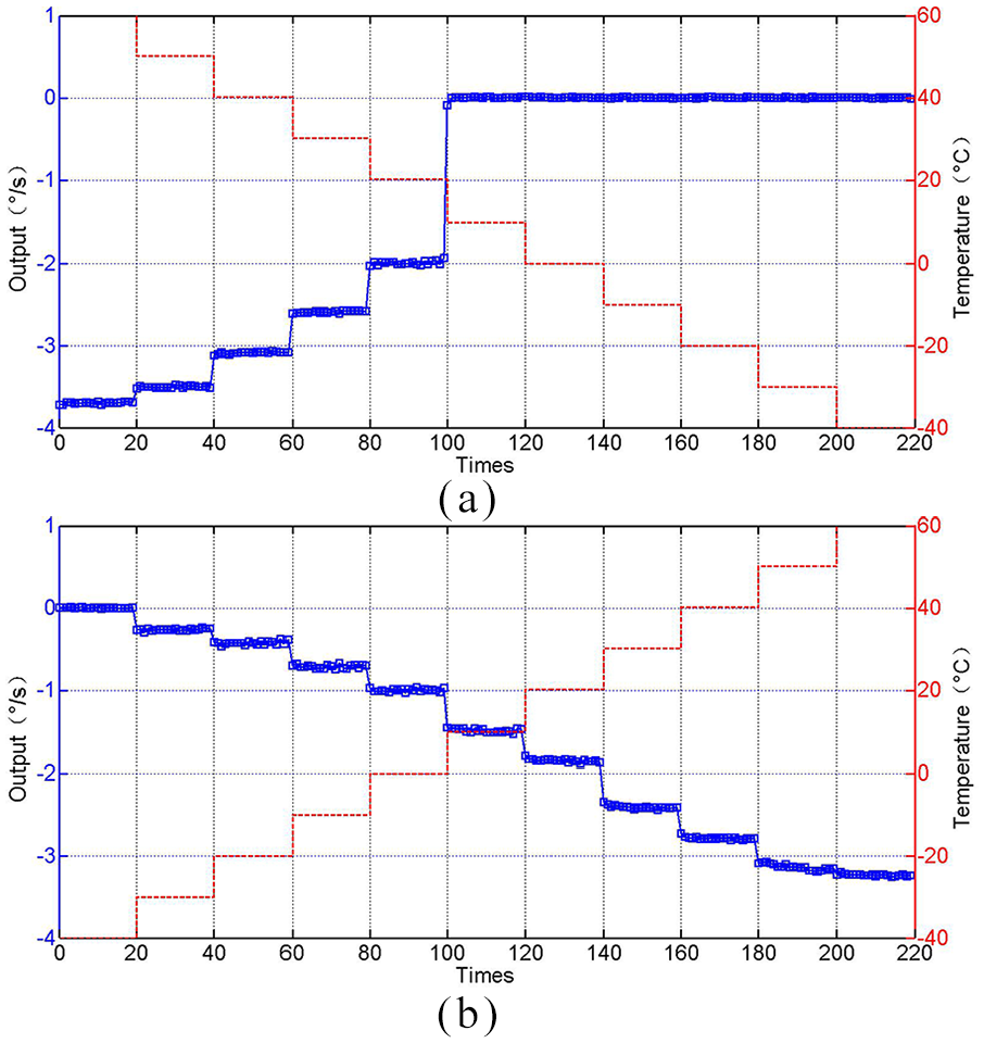
As for the test, the output data are shown in Figure 6. There are 2200 data points in each temperature experiment, with the majority of data points of the 220 data points are chosen to represent all data points (Figure 6). In order to improve the accuracy of C-SVM and SVM method, we add the output data of Y axis based on another MEMS gyroscope under the temperature experiment. The original data are shown in Figure 7, and Figure 8 includes 220 points of data.
The output data of MEMS gyroscope: (a)

The original output data of another MEMS gyroscope: (a) 60°C to −40°C and (b) −40°C to 60°C.

The output data of the MEMS gyroscope: (a) 60°C to −40°C and (b) −40°C to 60°C.
From Figures 9 and 10, we can see that the output of X axis varied a lot in the test. For the sake of reducing the temperature drift, SVM, an improved SVM algorithm method and the least square method are used in this article. From Figures 9 and 10, we also can see that the temperature drift model based on SVM algorithm, C-SVM algorithm, and the least square method are established.

The output of the MEMS gyroscope range from −40°C to 60°C.

The output of the MEMS gyroscope range from 60°C to −40°C.
From Figures 11 and 12, we can see that the output of Y axis varied a lot in the test. For the sake of reducing the temperature drift, SVM, an improved SVM algorithm method and the least square method are used in this article. From Figures 11 and 12, we also can see that the temperature drift model based on SVM algorithm, C-SVM algorithm, and the least square method are established.

The output of another MEMS gyroscope range from −40°C to 60°C.

The output of another MEMS gyroscope range from
Based on these temperature drift models, it can be easily recognized that the three curves which are the best algorithm to reduce the temperature drift. Obviously, C-SVM method is suitable to reduce the temperature drift.
Allan variance 17 was proposed to distinguish the various error sources which are used to evaluate the performance of MEMS gyroscopes nowadays. The temperature drift will be divided into mainly five parts and the most important parts which are N (Angle random walk) and B (Bias instability). The method results of Allan variance analysis based on X axis and Y axis are shown in Tables 2 and 3.
The method results of Allan variance analysis based on X axis.

SVM: support vector machine; C-SVM: C-means support vector machine.
The method results of Allan variance analysis based on Y axis.
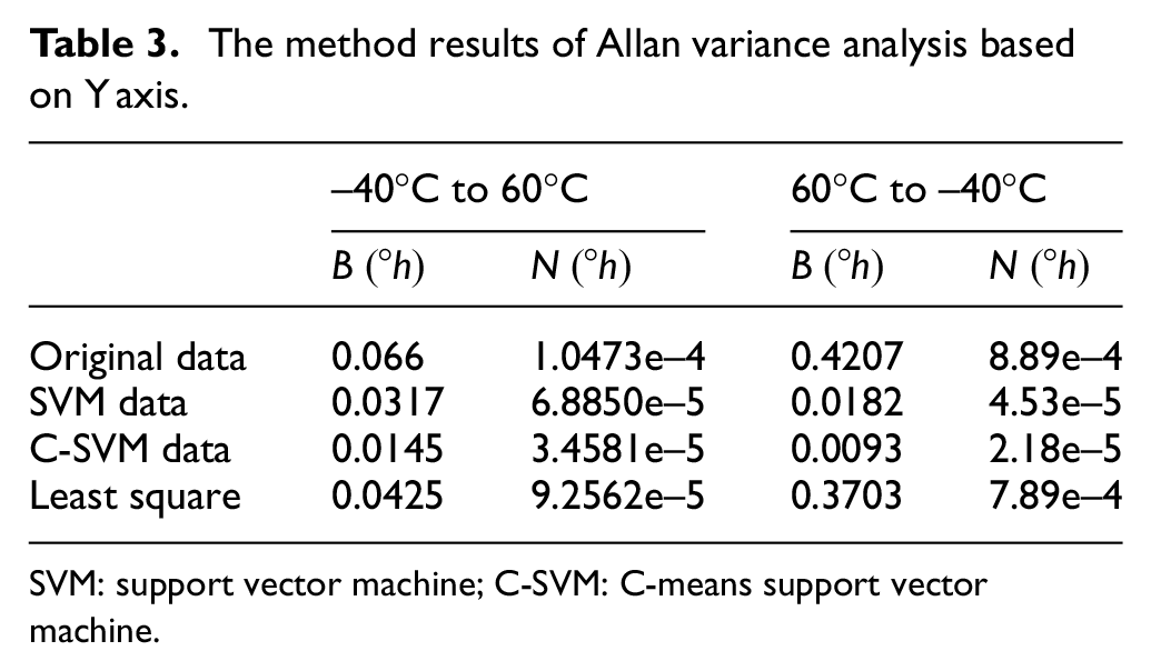
SVM: support vector machine; C-SVM: C-means support vector machine.
From Table 2, it can be seen that by using SVM and C-SVM methods, the factors of Allan variance analysis are reduced, which shows that C-SVM method is the better method.18–24 As for bias instability, when the temperature is ranged from −40°C to 60°C, the factor of B is reduced from 0.424
Conclusion
In this article, two methods are suggested to reduce the temperature drift, which are SVM method and C-SVM. As for bias instability, when the temperature is ranged from −40°C to 60°C, the factor of B is reduced from 0.424
Footnotes
Handling Editor: Antonio Lazaro
Declaration of conflicting interests
The author(s) declared no potential conflicts of interest with respect to the research, authorship, and/or publication of this article.
Funding
The author(s) disclosed receipt of the following financial support for the research, authorship, and/or publication of this article: This work is supported by the National Natural Science Foundation of China (grant no. 51705477), and Pre-Research Field Foundation of Equipment Development Department of China (grant no. 61405170104). The research is also supported by program for the Top Young Academic Leaders of Higher Learning Institutions of Shanxi, Fund Program for the Scientific Activities of Selected Returned Overseas Professionals in Shanxi Province, Shanxi Province Science Foundation for Youths (grant no. 201801D221195), Young Academic Leaders of North University of China (grant no. QX201809), and the Open Fund of State Key Laboratory of Deep Buried Target Damage (grant no. DXMBJJ2017-15).