Sage Journals: Discover world-class research

Abstract

To improve the control precision of the drive system of hydraulic tracked vehicles, we established a mathematical model of the drive system based on the analysis of structural characteristics of the high-clearance hydraulic tracked vehicles and the dual-pump dual-motor drive system and developed a control strategy based on the quantitative feedback theory. First, the mutual independence of the two motor channels was achieved through channel decoupling. Then, the loop-shaping controller and the pre-filter were designed for the two channels. The result of a simulation experiment indicates that the proposed control method is very effective in suppressing external uncertainties and smoothening the speed-switching process of the hydraulic motor. Finally, an hydraulic tracked vehicle steering experimental test was carried out. The results show that under two different steering modes, the maximum standard deviation of the output speeds of the inner and outer motors of the hydraulic tracked vehicle is only 0.42, which meets the performance requirement on the hydraulic motor speed. The average steering track radii of the geometric centers of the inner and outer tracks are 1.828 and 0.033 m, respectively, and the relative errors are 1.56% and 3.19%, respectively. This demonstrates that the proposed control method achieves satisfactory results in the robust control of the hydraulic tracked vehicle drive system. It provides some references for the future control research of the hydraulic servo drive system of the high-clearance hydraulic tracked vehicles.

Keywords

Hydraulic tracked vehicle drive system quantitative feedback theory uncertain system interference suppression robust control

Introduction

Because of the strong-grade ability, large ground-contact area, mild soil-compaction effect, and high stability, the use of high-clearance hydraulic tracked vehicles (HTVs) has been widely increasing in small patches of farmland and hilly areas for fertilization, weeding, and pesticide spraying purposes. High labor intensity and poor working environment characterize vehicle-based farming activities related to high stalk crops. In particular, the health of the operator is put at risk during the pesticide spraying operation due to the easy-to-spread nature of pesticide sprays.¹ Therefore, developing highly automated tracked vehicles has become a trend in the research field of agriculture machinery. Simple and compact structure and high reliability are the basic requirements of vehicle automation. To ensure the controllability and operability of the vehicles, a coupling control strategy of force and displacement,^2–4 a H-extension controller based on active front steering system in extreme conditions,⁵ and optimally adapt automatic control of intelligent electric vehicles to driving styles⁶ had been proposed successively by some experts. With the development of technology and the ever-higher expectation of the users on the control performance of tracked vehicles, some techniques like these will be increasingly used in agricultural tracked vehicles.

The electro-hydraulic servo system, combining the advantages of electronic and hydraulic control, is characterized by high control precision, fast response, high torque output, and flexible signal processing, and the ease of implementing feedbacks of various parameters, and it is a good choice to realize the automation of agricultural tracked vehicle drive system. However, because of several factors such as the oil compressibility, nonlinear friction, time variation, possible load disturbances, and unpredictable parameter perturbation, the hydraulic servo system may not fulfill its purpose of high-precision control.^7,8 To explore how to enable robust control with the hydraulic servo system under the negative influence of model uncertainty, some scholars have developed adaptive fuzzy proportional-integral-derivative (PID) algorithm for online real-time adjustment of PID parameters,⁹ the genetic algorithm for adaptive adjustment of PID control parameters,¹⁰ the anti-interference adaptive control scheme based on full-state feedback,¹¹ the sliding mode controller which is immune from the influence of parameter variation and external disturbances of electro-hydraulic servo system,¹² the model reference adaptive controller (MRAC) based on mathematical model,¹³ and the adaptive neural network controller,¹⁴ effectively improving the steady-state control precision and dynamic response speed. There also have been developed some hybrid controllers such as an adaptive integral back-stepping controller,¹⁵ a novel sliding mode controller,¹⁶ and predictive controllers.¹⁷ However, hydraulic servo systems are time-varying systems. As the conventional control methods are usually suitable for slow time-varying systems, most of them are too complicated to be directly applied to hydraulic servo systems^18,19 due to poor transient response performance under complicated working conditions.^20,21 Therefore, it is especially necessary to develop control strategies suitable for tracked vehicle hydraulic servo systems.

Quantitative feedback theory (QFT) is a robust controller design method especially suitable for systems with uncertainties.^22,23 In the practice of control system design, applying QFT helps maintain the balance between various performance indicators of the system, which provides an effective method for adjusting the controller. Initially, the QFT was used in the design of the flight control system;²⁴ at present, its application has expanded to many fields such as process control,²⁵ vehicle control,^26,27 robot control, wind power system control,^28,29 and spacecraft control.³⁰

This study applies the QFT to develop a drive system control strategy based on the analysis of structural characteristics of the high-clearance HTVs and the dual-pump dual-motor drive system. The proposed control strategy aims at solving some steering-related control problems caused by parameter uncertainties, time-varying, and nonlinear nature of the hydraulic drive system. First, a mathematical model of the drive system was established, and the mutual independence of the two motor channels was achieved through channel decoupling. Then, the loop-shaping controller and the pre-filter were designed for the two channels. The simulation results prove that the proposed control method is very effective in suppressing external uncertainties and outperforms the conventional PID control method in smoothening the speed-switching process of a hydraulic motor. The results of an HTV steering experiment show that the proposed control method enables high-precision steering in two steering modes, fulfilling its purpose of providing a robust control for the drive system of tracked vehicle.

System modeling and analysis

Description of the drive system of the tracked vehicle

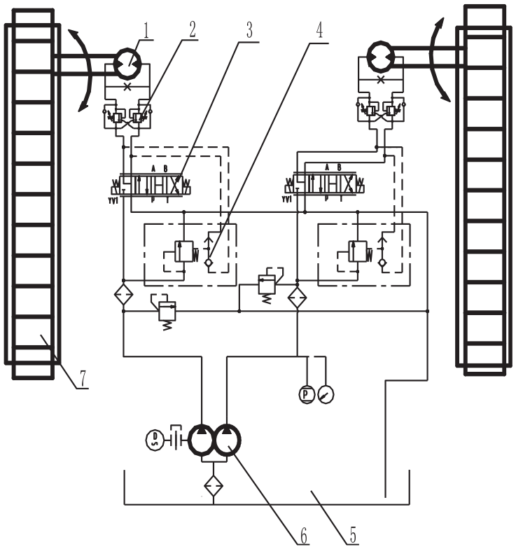
Figure 1 shows the drive system of the tracked vehicle. The drive system uses a dual-pump dual-motor throttle governing circuit; it is a typical electro-hydraulic servo valve-controlled motor system. The drive system mainly consists of engine, double pump, hydraulic motor, servo valve, balance valve, and three-way compensator. According to the figure, two hydraulic motors (1) are connected with the two corresponding tracks (7). When the tracked vehicle is moving, the movement direction can be controlled by adjusting the speeds of the two motors, and the speed of each motor can be adjusted by changing the opening of the corresponding servo valve. The drive system can drive the tracked vehicle to perform various actions ranging from moving in a straight line to in-situ steering.

Figure 1.

Drive system of the tracked vehicle.

Mathematical model of the tracked vehicle drive system

To design a robust controller for the tracked vehicle drive system, it is necessary to establish a mathematical model of the drive system at first. The model consists of a hydraulic servo system mathematical model and a tracked vehicle dynamics model.

Mathematical model of the hydraulic servo system

The tracked vehicle drive system consists of two symmetrical four-way valve-controlled motor oil circuits. The linearized flow equations for the servo valve ports are

Q_{L 1} = K_{q 1} x_{v 1} - K_{C 1} P_{L 1}

(1)

Q_{L 2} = K_{q 2} x_{v 2} - K_{C 2} P_{L 2}

(2)

The hydraulic motor flow continuous equations are

Q_{L 1} = D_{m 1} θ'_{m 1} + C_{t 1} P_{L 1} + \frac{V_{t 1}}{4 β_{e}} P'_{L 1}

(3)

Q_{L 2} = D_{m 2} θ'_{m 2} + C_{t 2} P_{L 2} + \frac{V_{t 2}}{4 β_{e}} θ'_{L 2}

(4)

The moment balance equations of hydraulic motors are

D_{m 1} P_{L 1} = J_{1} {θ ″}_{m 1} + T_{1}

(5)

D_{m 2} P_{L 2} = J_{2} {θ ″}_{m 2} + T_{2}

(6)

where Q_L is the load flow of servo valve, X_v is the spool displacement of servo valve, K_q is the flow gain of servo valve, K_c is the flow pressure coefficient of servo valve, P_L is the load pressure drop, D_m is the hydraulic motor’s displacement, θ_m is the rotation angle of hydraulic motor, C_t is the leakage coefficient of hydraulic motor, V_t is the total volume of the two chambers of the hydraulic motor and the connected pipes, J₁ and J₂ are the inertia values of hydraulic motors, respectively, β_e is the oil volume elastic modulus, and T is the external load moment applied to the hydraulic motor shaft.

Dynamics model of the tracked vehicle

Moving in a straight line and in-situ steering are the critical points of the steering motion of the tracked vehicle, so it is only necessary to establish the steering dynamics model of the tracked vehicle. The force condition of the tracked vehicle is relatively complicated during steering movement.^31,32,33 For the convenience of analysis, this study makes the following assumptions

The center of mass of the tracked vehicle coincides with the geometric center.

The pressure of the track is evenly distributed across the ground-contact area, and the influence of the track’s width is ignored.

As the speed of the tracked vehicle is low, the air resistance and the centrifugal force are ignored.

The shearing resistance and bulldozing resistance of the tracked vehicle are ignored. Thus, a simplified steering movement model of the tracked vehicle is established (Table 1).

Table 1.

Parameters of the tracked vehicle.

Symbol	Parameter
V ₁, V₂	Inner and outer track speeds (m/s)
V_c	Speed of the tracked vehicle center (m/s)
R	Turning radius of the tracked vehicle (m)
ω	Steering angular speed of the tracked vehicle (rad/s)
F ₁, F₂	Traction or braking forces at the ground-contact areas of inner and outer tracks (N)
F_R ₁, F_R₂	Ground friction resistance received by inner and outer tracks (N)
M_μ	Steering resistance moment (N m)
B	Distance between track centers (m)
L	Track ground-contact length (m)
C, C ₁, C₂	Tracked vehicle center, steering centers of inner, and outer tracks
O	Tracked vehicle steering center
G	Tracked vehicle gravity (N)
μ	Steering drag coefficient
f	Ground deformation resistance coefficient
J	Moment of inertia of the tracked vehicle

According to Figure 2, the steering motion of the tracked vehicle can be decomposed into a component parallel to the motion of the vehicle plane center C and a component circling the center C, and steering is realized by creating a speed difference between the two tracks at the two sides. When the inner and outer tracks are rolling in the same direction at the same speed, the tracked vehicle is moving in a straight line. When the inner and outer tracks are rolling in opposite directions with the same speed, the tracked vehicle is doing in-situ steering. Given that the tracked vehicle experiences different force conditions in different driving states, the steering motions can be divided into two types: R ≥ B/2 and 0 ≤ R < B/2.

Figure 2.

The two types of steering motion of the tracked vehicle: (a) (R ≥ B/2) and (b) (0 ≤ R < B/2).

When the tracked vehicle is turning, the theoretical steering radius can be calculated using equation (7) if no slipping occurs during steering

R = \frac{B}{2} \cdot \frac{v_{2} + v_{1}}{v_{2} - v_{1}}

(7)

The speeds and steering angular speeds of the two tracks during steering are

v_{1} = v_{c} - ω \cdot \frac{B}{2}

(8)

v_{2} = v_{c} + ω \cdot \frac{B}{2}

(9)

ω = \frac{V_{C}}{R}

(10)

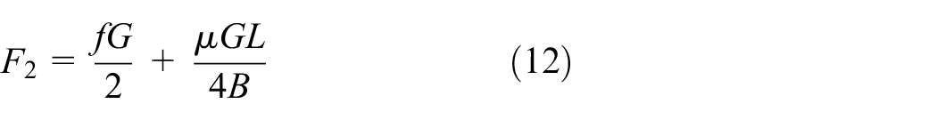
When R ≥ B/2, both the inner and outer tracks are rolling in the same direction (see Figure 2(a)). The braking force F₁ of the inner track and the traction force F₂ of the outer track can be expressed as

F_{1} = \frac{fG}{2} - \frac{μ GL}{4 B}

(11)

F_{2} = \frac{fG}{2} + \frac{μ GL}{4 B}

(12)

When 0 ≤ R < B/2, both the inner and outer tracks are rolling in opposite directions, and the rolling direction of the outer track is consistent with that of the vehicle (see Figure 2(b)). At this time, the driving forces applied to the inner and outer tracks are of the same magnitude and opposite directions. The expressions of the driving forces are

F_{1} = - \frac{fG}{2} - \frac{μ_{max} GL}{4 B}

(13)

F_{2} = \frac{fG}{2} + \frac{μ_{max} GL}{4 B}

(14)

When the tracked vehicle is turning at a radius of R ≥ B/2, the dynamic balance equation is

mv' = F_{1} + F_{2} - F_{R 1} - F_{R 2}

(15)

J ω' = (F_{2} - F_{1} + F_{R 1} - F_{R 2}) \frac{B}{2} - M_{μ}

(16)

When the tracked vehicle is turning at a radius of 0 ≤ R < B/2, the inner and outer tracks are rolling in opposite directions. As a result, the driving force and the frictional force of the inner track are also reversed. So, the dynamic balance equation of the tracked vehicle turning at a radius of 0 ≤ R < B/2 can be obtained by adding negative signs in front of F₁ and F_R₁

F_{R} = fG

(17)

μ = \frac{μ_{max}}{0.925 + 0.15 \frac{R}{B}}

(18)

M_{μ} = \frac{μ GL}{4}

(19)

Parameter equation of hydraulic motor

When the tracked vehicle is not experiencing slipping during driving, the torque is

T_{i} = \frac{F_{i} r}{i η}

(20)

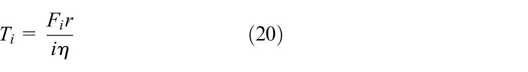
where i = 1, 2. T₁ and T₂ correspond to the torques of the inner motor and outer motor, respectively (N m), i is the side transmission ratio, η is the efficiency of the section from the motor output shaft to the track, and r is the driving wheel radius (m).

The relationship between the motor speed and the steering angular speed when the tracked vehicle is turning can be obtained using equations (8) and (9)

v_{c} = \frac{r}{2} (θ'_{m 1} + θ'_{m 2})

(21)

ω = \frac{r}{B} (θ'_{m 2} - θ'_{m 1})

(22)

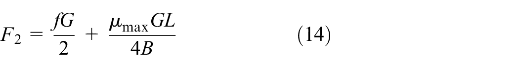
When the tracked vehicle is turning at a radius of R ≥ B/2, the driving force can be calculated using equations (15) and (16)

F_{1} = (\frac{m {v'}_{c}}{2} - \frac{J ω'}{B}) - \frac{M_{μ}}{B} + F_{R 1}

(23)

F_{2} = (\frac{m {v'}_{c}}{2} + \frac{J ω'}{B}) + \frac{M_{μ}}{B} + F_{R 2}

(24)

The torque balance equations of hydraulic motors can be obtained using equations (20)–(24)

T_{1} = [(\frac{mr}{4} + \frac{Jr}{B^{2}}) {θ ″}_{m 1} + (\frac{mr}{4} - \frac{Jr}{B^{2}}) {θ ″}_{m 2} - \frac{μ GL}{4 B} + F_{R 1}] \frac{r}{i η}

(25)

T_{2} = [(\frac{mr}{4} + \frac{Jr}{B^{2}}) {θ ″}_{m 1} + (\frac{mr}{4} - \frac{Jr}{B^{2}}) {θ ″}_{m 2} + \frac{μ GL}{4 B} + F_{R 2}] \frac{r}{i η}

(26)

Similarly, when the tracked vehicle is turning at a radius of 0 ≤ R < B/2, the torque equations of the hydraulic motors are

T_{1} = [(\frac{Jr}{B^{2}} - \frac{mr}{4}) {θ ″}_{m 2} - (\frac{mr}{4} + \frac{Jr}{B^{2}}) {θ ″}_{m 1} + \frac{μ_{max} GL}{4 B} + F_{R 1}] \frac{r}{i η}

(27)

T_{2} = [(\frac{mr}{4} + \frac{Jr}{B^{2}}) {θ ″}_{m 1} + (\frac{mr}{4} - \frac{Jr}{B^{2}}) {θ ″}_{m 2} + \frac{μ_{max} GL}{4 B} + F_{R 2}] \frac{r}{i η}

(28)

Design of QFT controller

In this study, the controller is designed based on QFT. First, the uncertain parameter disturbances and external disturbances of the drive system during the driving process are identified. Then, the system parameter uncertainties and system performance indicators are presented on the Nichols chart as robust stability boundary, tracking boundary, and interference suppression boundary quantitatively, creating the condition for a comprehensive analysis of the drive system of the tracked vehicle.

Design of the system decoupling controller

Given that a strong coupling effect exists in the drive system, the design of a QFT controller for the drive system is difficult because the coupling effect makes it challenging to determine the boundaries of QFT parameter uncertainties. Besides, converting a multiple-input multiple-output (MIMO) system into a single-input single -output (SISO) system increases the difficulty in the design. Therefore, we decided to decouple the drive system before designing a QFT controller for it. For the R ≥ B/2 steering state of the tracked vehicle, a decoupling control matrix is designed to isolate the interference between the two inputs and the two outputs. The same decoupling method is applied to the 0 ≤ R < B/2 steering state. After the drive system model (equations (25) and (26) undergoes the Laplace transform, the decoupled drive system is obtained (see Figure 3)).

{\begin{matrix} G_{p 11} = \frac{\frac{D_{m}}{(K_{C 1} + C_{t 1}) + \frac{V_{t 1}}{4 B_{e}} s}}{(1 + \frac{mr}{4} + \frac{Jr}{B^{2}}) s^{2}} = \frac{D_{m}}{\frac{V_{t 1}}{4 B_{e}} (1 + \frac{mr}{4} + \frac{Jr}{B^{2}}) s^{3} + (K_{C 1} + C_{t 1}) (1 + \frac{mr}{4} + \frac{Jr}{B^{2}}) s^{2}} \\ G_{p 22} = \frac{\frac{D_{m}}{(K_{C 2} + C_{t 2}) + \frac{V_{t 2}}{4 B_{e}} s}}{(1 + \frac{mr}{4} - \frac{Jr}{B^{2}}) s^{2}} = \frac{D_{m}}{\frac{V_{t 2}}{4 B_{e}} (1 + \frac{mr}{4} - \frac{Jr}{B^{2}}) s^{3} + (K_{C 2} + C_{t 2}) (1 + \frac{mr}{4} - \frac{Jr}{B^{2}}) s^{2}} \\ G_{P 12} = \frac{mr}{4} - \frac{Jr}{B^{2}} \\ G_{p 21} = \frac{mr}{4} + \frac{Jr}{B^{2}} \end{matrix}

(29)

[\begin{matrix} θ_{m 1} \\ θ_{m 2} \end{matrix}] = [\begin{matrix} G_{P 11} \\ 0 \end{matrix} \begin{matrix} 0 \\ G_{P 22} \end{matrix}] [\begin{matrix} Q_{L 1} \\ Q_{L 2} \end{matrix}]

(30)

Figure 3.

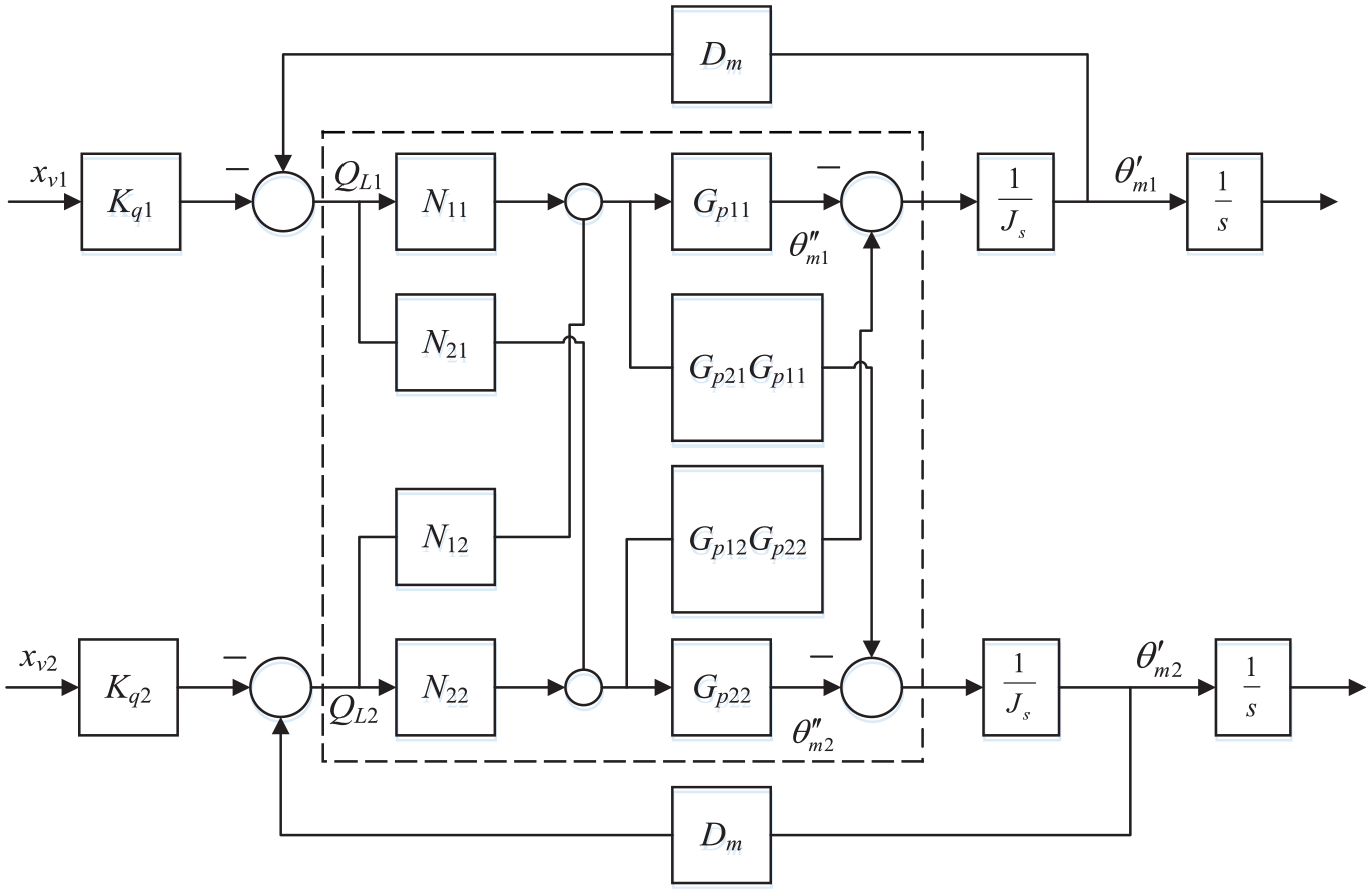
Block diagram of drive system decoupling.

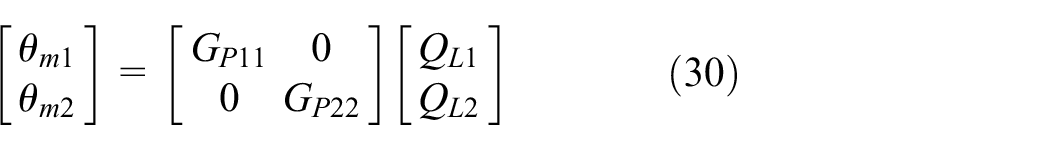
The goal is to design a matrix to satisfy the following equation

[\begin{matrix} G_{P 11} \\ G_{P 21} \end{matrix} \begin{matrix} G_{P 12} \\ G_{P 22} \end{matrix}] [\begin{matrix} N_{11} \\ N_{21} \end{matrix} \begin{matrix} N_{12} \\ N_{22} \end{matrix}] = [\begin{matrix} G_{P 11} \\ 0 \end{matrix} \begin{matrix} 0 \\ G_{P 22} \end{matrix}]

(31)

Analysis of QFT controller design

The implementation of the above decoupling process allows achieving the mutual independence of the two motor channels. Now, we need to design a QFT controller for each motor channel to meet the performance robustness requirements of the drive system in the presence of parameter perturbation. Thus, a control model that aims at solving the parameter uncertainty and input perturbation uncertainty problems in the tracked vehicle drive system model is designed (Figure 4). A loop-shaping controller and a pre-filter are also designed for the controller.

Figure 4.

Structure of robust control model based on QFT.

Design requirements and robust boundaries

Considering the actual operations of the tracked vehicle, three main system performance boundaries are needed, that is, robust stability margin, anti-interference performance, and servo tracking robust performance. The first thing that needs to be considered is that the bandwidth of the entire system should be determined by the power mechanism, and the bandwidth of the servo valve is much wider than that of the motor power mechanism. The natural frequency of the motor of the hydraulic drive system calculated using equation (32) is 18.2658 rad/s. Considering that the actual load includes the track and its transmission mechanism, the bandwidth of the actual power mechanism should be lower.

ω_{h} = \sqrt{\frac{4 B_{e} D_{m}^{2}}{V_{t} J_{m}}}

(32)

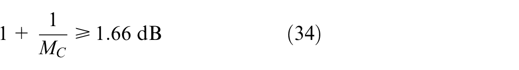
Robust stability margin

| \frac{G_{p} (j ω) G_{QFT} (j ω)}{1 + G_{p} (j ω) G_{QFT} (j ω)} | \leq M_{c}

(33)

This indicator is used to ensure the stability margin of the system within the entire operating frequency band. Considering the general stability margin of the electro-hydraulic servo control system of the tracked vehicle, the amplitude margin is determined to be around 1.66 dB, and the phase margin is about 50°, which can meet the requirements of most working conditions. According to the empirical formula, the value of M_c is about 1.2

1 + \frac{1}{M_{C}} \geq 1.66 dB

(34)

180 ° - 2 \arccos (\frac{0.5}{M_{C}}) \geq 50 °

(35)

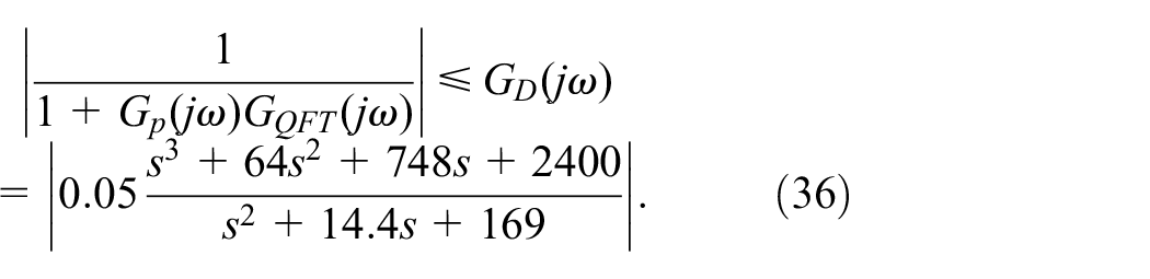
Anti-interference performance

Anti-interference performance indicators include output disturbance robustness and input disturbance robustness. From an analysis of the mathematical model of the output disturbance robustness, the external disturbance is attenuated at the rate of 40 dB per 10 octaves in the high-frequency band. So the transfer function is defined to rise at a rate of 40 dB per 10 octaves. Defining the robust performance boundaries can effectively suppress external disturbances lower than 3 Hz

\begin{matrix} | \frac{1}{1 + G_{p} (j ω) G_{QFT} (j ω)} | \leq G_{D} (j ω) = | 0.05 \frac{s^{3} + 64 s^{2} + 748 s + 2400}{s^{2} + 14.4 s + 169} | \end{matrix}

(36)

The input disturbance robustness is used to ensure the robustness of the output under the influence of the system input interference signal. Here

M_{in} = 0.01 dB

(37)

Servo tracking robustness

By considering the actual operation of the tracked vehicle, the step response is used to constrain the servo performance

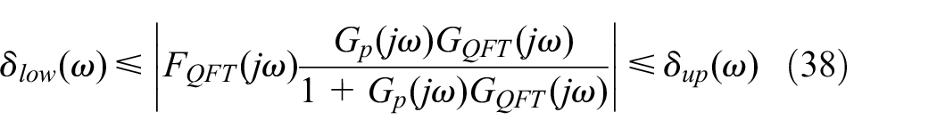
δ_{low} (ω) \leq | F_{QFT} (j ω) \frac{G_{p} (j ω) G_{QFT} (j ω)}{1 + G_{p} (j ω) G_{QFT} (j ω)} | \leq δ_{up} (ω)

(38)

The step response performance indicators of the system within the frequency bandwidth are

Rise time: T_r =1 s

Overshoot: M = 10%

Adjustment time: T_s = 2 s

Design of controller

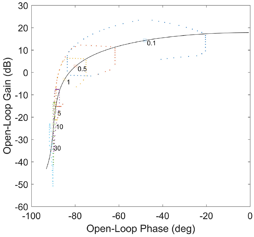
Generating a design template

Given the setting of the parameter uncertainty, the QFT design template shown in Figure 5 can be obtained. The frequencies ω = 0.1, 0.5, 1, 5, 10, and 30 rad/s are selected on the Nichols chart.

Figure 5.

Template of drive system at selected frequencies on the Nichols chart.

Synthesis of performance boundaries

The overall design boundary of the QFT controller can be obtained by synthesizing the robust stability margin specification, robust output disturbance specification, and robust input disturbance specification. Gains, zero poles, and complex poles are added to the model to ensure (1) the low-frequency open-loop Nichols curve of the system is above and as close as possible to the constraint boundary of the response frequency point and (2) the amplitude–phase curve of the high-frequency section is outside the robust stability boundary. Figure 6 shows the resulting corrected system Nichols chart. The system performance is above the boundary at all frequency points, and the minimum gain is guaranteed. The resulting controller transfer function is

G_{c} (s) = \frac{21.7023}{\frac{s^{2}}{{115.2}^{2}} + 2 \times \frac{0.97 s}{115.2} + 1}

(39)

Figure 6.

Open-loop frequency response and QFT boundaries.

Performance check

The results are fed into the transfer function model for verification to make the results more reliable. The stability margin robustness, output anti-disturbance robustness, and input anti-disturbance robustness are verified separately. The results are shown in Figures 7 –9, respectively. The dotted lines in the graphs represent the performance indicators set in equations (33)–(37); the corrected system can meet the set performance requirements very well.

Figure 7.

Stability margin robustness verification diagram.

Figure 8.

Output anti-disturbance robustness verification diagram.

Figure 9.

Input anti-disturbance robustness verification diagram.

Design of pre-filter

Considering that the system has the tracking capability, it is necessary to design a pre-filter for it. From the Bode diagram of Figure 10, the closed-loop frequency response boundary of the system is within the tracking performance boundary under the parameter disturbance condition. Thus, the transfer function of the pre-filter is

G_{F} = 0.0683 \times \frac{s + 50.07}{s + 3.292}

(40)

Figure 10.

Design curve of pre-filter.

Simulation analysis

A simulation experiment on the motor channels was performed to verify the effectiveness of the proposed control strategy, the results were analyzed, and then the proposed control strategy was compared with the conventional PID control method. The necessary parameters can be calculated using equations (1)–(28). Table 2 lists the key parameters of the drive system.

Table 2.

Key parameters of the tracked vehicle drive system.

Parameter	Numerical value
Tracked vehicle mass (m/kg)	500
Moment of inertia of vehicle (J/kg m²)	550
Body width (B/m)	1.2
Track length (L/m)	1.22
Radius of motor drive wheel(r/m)	0.095
Rolling friction coefficient, f	0.05
Steering drag coefficient, μ	0.6
Overall efficiency of hydraulic motor and transmission mechanism η	0.63
Side transmission ratio, i	1
Servo valve flow gain (K_q/s V)	0.013
Servo valve flow pressure coefficient, K_c/m³/s Pa	2.06271 × 10⁻¹⁰
Hydraulic motor leakage coefficient, C_t	2.5 × 10⁻¹²
Oil volume elastic modulus, β_e	1000
Hydraulic motor inertia (J_i/kg/m³)	10
Oil density (ρ/kg/m³)	850

As shown in Figures 11 and 12, simulation analysis is performed for R ≥ B/2 and 0 ≤ R < B/2 steering states of tracked vehicles, and the comparison of response state and robust performance is obtained under the action of different controllers. In the simulation, an impulse signal with the size of 50 N m and the duration of 0.1 s was added to one side of motor passage at 5 s. It can be seen from the figure that compared with PID control, the change value of motor speed is small under the action of QFT controller, only about one-fifth of the change value under PID control, and the impulse signal has little impact on the motor speed of another passage; the change of motor torque value is little, which can recover in less time with less overshoot; the instantaneous turning radius change value of the tracked vehicle is only about one-fifth of that under PID control. The simulation results show that under the same parameter perturbation condition, QFT controller can suppress the perturbation in a short time and show a high robust performance.

Figure 11.

R ≥ B/2 steering states.

Figure 12.

0 ≤ R < B/2 steering states.

Experiment on steering performance of the tracked vehicle

A steering experiment was conducted to test the reliability of the robust control of the tracked vehicle drive system when the vehicle is performing R ≥ B/2 steering and 0 ≤ R < B/2 steering. In order to obtain good test results, the tests were carried out on a patch of brick-paved hard ground to increase the friction between the tracks and the ground, thus avoid slipping. The main instruments and tools used in the test include an encoder, tape measure, marking line, Jisibao G970 high-precision GNSS device, Bluetooth module, embedded board, and portable computer. During the test, the encoders mounted on the rear wheels collected the speeds of the two hydraulic motors, and the embedded board capable of Hampel filtering integrated the data before transferring the information to the computer. A vehicle-mounted portable computer-controlled the servo valve-controlled motor system. The tracked vehicle was positioned in real-time using the Jisibao G970 high-precision GNSS device to obtain its motion track during the test. A Bluetooth module transmitted the position data to the vehicle-mounted computer, and the computer processed the position data, obtaining the motion track of the vehicle. Figure 13 shows the test site.

Figure 13.

The actual test site.

Analysis of motor output speed

The R ≥ B/2 steering test was carried out under the following conditions: the inner and outer motors were turning in the same direction at the speeds of 50 and 100 r/min, respectively, and the rotational speeds were 50 and 100 r/min, respectively. The 0 ≤ R < B/2 steering test was conducted under the following conditions: the inner and outer motors were turning in the opposite directions at the same speed of 50 r/min (the theoretical turn radius is 0). According to equations (7)–(10), it would take about 15 s for the tracked vehicle to make a 360° turn in the R ≥ B/2 steering test, and 8 s in the 0 ≤ R < B/2 steering test. When the tracked vehicle was turning, the E6B2-CWZ6C encoder collected the hydraulic motor speed signal that was then output by the embedded board (the signal processing frequency was set to 2 Hz).

The motor output speed is stable under the two steering conditions, and the speeds of the inner and outer motors are close to the theoretical values (Table 3). In the two steering tests, the average output speeds of the inner and outer motors are slightly lower than the set speeds due to the uncertain nature of the road surface resistance, but the discrepancies between the actual and the set values were small (the standard deviation was only 0.42) and the output speed was stable. This result demonstrates that the controller has a good robust performance in the presence of system parameter perturbation and uncertainty.

Table 3.

Speed parameters of the two hydraulic motors during steering test.

Parameter	Differential steering		In-situ steering
Parameter	Inner motor	Outer motor	Inner motor	Outer motor
Theoretical value	50	100	50	−50
Mean	49.83	99.90	49.55	−49.92
Standard deviation	0.40	0.34	0.42	0.34
Coefficient of variation	0.80%	0.33%	0.80%	0.68%

Analysis of steering track

In order to ensure that enough information points could be collected during the test, the sampling frequency of the G970 system was set to 5 Hz. Furthermore, the static data collection was performed under the idle condition to verify the positioning accuracy. The test results show that the test data points are all distributed in a circle with a diameter of 2 cm, indicating that the measurement accuracy is high enough to meet the test requirement. The steering position data were transmitted to the vehicle-mounted portable computer via the Bluetooth module and stored in the computer. Later, the latitude and longitude values were extracted from the track information and converted using the Gaussian projection calculation formula and sorted based on which the turning circle was obtained through the fitting with MATLAB. Figure 14 illustrates the installation location of the mobile station, where O and O₁ are the geometric center of the ground-contact area of the tracked vehicle and the phase center of the mobile station, respectively. The distances between the phase center and the geometric centers a and b are 0.568 and 0.538 m, respectively, and the phase center is 1.6 m high from the ground. Equations (41) and (42) describe the relationship between the turning track radius of the geometric center of the ground-contact area and the turning track radius of the mobile station phase center.

R_{R \geq B / 2} = \sqrt{R_{n 1}^{2} - a^{2}} - b

(41)

R_{0 \leq R < B / 2} = R_{n 2} - \sqrt{a^{2} + b^{2}}

(42)

where a is the longitudinal distance between the phase center of the mobile station and the geometric center of the ground-contact area of the tracked vehicle (a = 0.586 m), b is the transverse distance between the phase center of the mobile station and the geometric center of the ground-contact area of the tracked vehicle (b = 0.538 m), R_R≥B/₂ is the turning track radius of the geometric center of the ground-contact area when the tracked vehicle is performing R ≥ B/2 steering, R_R_≤B/2 is the turning track radius of the geometric center of the ground-contact area when the tracked vehicle is performing 0 ≤ R < B/2 steering, R_n₁ is the turning track radius of the mobile station phase center when the tracked vehicle is performing R ≥ B/2 steering, and R_n₂ is the turning track radius of the mobile station phase center when the tracked vehicle is performing 0 ≤ R < B/2 steering.

Figure 14.

Installation of mobile station.

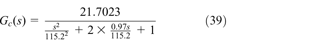
Figure 15 shows the turning tracks of the tracked vehicle; the vehicle slips and slides during in-situ steering process due to the high angular speed.

Figure 15.

Turning tracks of the tracked vehicle: (a) R ≥ B/2 and (b) 0 ≤ R < B/2.

Table 4 lists the parameters of the turning track of the vehicle. The average turning track radii of the geometric centers of the inner and outer tracks are 1.828 and 0.033 m, respectively, and the relative errors are 1.56% and 3.19%, respectively. The smallness of the relative error demonstrates that the vehicle turns on the brick-paved hard ground with satisfactory performance, meeting the design requirements of the tracked vehicle.

Table 4.

Turning parameters of the tracked vehicle.

Steering type	S/N of turning track	Steering track of receiver phase center			Steering track radius of geometric frame center
Steering type	S/N of turning track	Circle center abscissa (m)	Circle center ordinate (m)	Radius (m)	Value of each group (m)	Mean	Theoretical value (m)	Relative error
R ≥ B/2	1	−0.003	−0.023	2.436	1.826	1.828	1.8	1.56%
R ≥ B/2	2	−0.015	−0.025	2.439	1.830	1.828	1.8	1.56%
0 ≤ R < B/2	1	−0.006	−0.002	0.833	0.037	0.033	0	3.19%
0 ≤ R < B/2	2	0.026	0.020	0.824	0.028	0.033	0	3.19%

Conclusion

We have developed a QFT-based drive system controller based on an analysis of the structural characteristics of the high-clearance HTVs and the dual-pump dual-motor drive system. The proposed drive system controller is easy to implement, can improve the robust stability and dynamic tracking performance of the tracked vehicle drive system, and has good robust performance in the presence of system parameter perturbation and uncertainty. The simulation results show that the proposed control method barely generates oscillation and has a small overshoot when the control signal changes, outperforming the conventional PID control method. The results of the steering experiment show that the tracked vehicle can turn very well on the brick-paved hard ground, indicating that the controller achieves robust high stability by effectively suppressing the dynamic interference of the road surface. Facts have proved that QFT controller is feasible and stable for the hydraulic servo drive system of tracked vehicles, and it can be used as a reference basis for the research of control algorithms for hydraulic servo drive systems of the high-clearance HTVs.

Further work will be carried out in the following areas: the cross-coupling method is used to synchronize the two motor channels of the tracked vehicle, and the double closed-loop control method is used to further improve the control accuracy of the tracked vehicle during walking.

Footnotes

Handling Editor: Wei-Chiang Hong

Declaration of conflicting interests

The author(s) declared no potential conflicts of interest with respect to the research, authorship, and/or publication of this article.

Funding

The author(s) disclosed receipt of the following financial support for the research, authorship, and/or publication of this article: The study was supported by the Special project for the construction of Supported by China Agriculture Research System (grant no. CARS-03), Special project of modern agricultural industry technology system in Henan (grant no. S2019-02-G07), and Key Scientific Research Project of Henan Province Higher Education (grant no. 20A210029). We wish to acknowledge them for their support.

ORCID iD

Wanzhang Wang

References

Zhou

Shen

Qin

, et al. Research on the control efficiency of an autonomous self-propelled high clearance boom sprayer. Jiang Su Agri Mech 2006; 21(3): 22–25.

Zhao

Zhang

. Displacement and force coupling control design for automotive active front steering system. Mech Syst Signal Pr 2018; 106(2): 76–93.

Zhao

Zhang

. Coupling control strategy of force and displacement for electric differential power steering system of electric vehicle with motorized wheels. IEEE T Veh Technol 2018; 67(9): 8118–8128.

Zhao

Qin

Wang

, et al. Yaw and lateral stability control for four-wheel steer-by-wire system. IEEE/ASME T Mechatron 2018; 23(6): 2628–2637.

Zhao

Fan

Wang

, et al. H-infinity/dextension stability control of automotive active front steering system. Mech Syst Signal Pr 2019; 115: 621–636.

Alberto

, et al. Driving-style-based co-design optimization of an automated electric vehicle: a cyber-physical system approach. IEEE T Ind Electron 2019; 66(4): 2965–2975.

Yang

Zheng

Lan

, et al. Adaptive robust control for spatial hydraulic parallel industrial robot. Procedia Eng 2011; 15(1): 331–335.

Chalupa

Novak

. Modeling and model predictive control of a nonlinear hydraulic system. Comput Math Appl 2013; 66(2): 155–164.

Yao

Deng

. Active disturbance rejection adaptive control of hydraulic servo systems. IEEE T Ind Electron 2017; 64(10): 8022–8032.

10.

Qiao

Zhang

Yan

. Design and simulation of adaptive fuzzy PID for electro-hydraulic servo system. Mod Mach Tool Automat Manuf Tech 2018; 534(8): 136–138, 148.

11.

Zhang

. Application of improved genetic algorithm PID controller in electro-hydraulic servo system. Proces Autom Instrum 2017; 3808: 28–32.

12.

You

. Load rigidity adaptive control of electro-hydraulic servo universal testing machine force control system. Control Theory Appl 2018; 35(4): 11–19.

13.

Huang

. System-decomposition-based multilevel control for hydraulic press machine. IEEE T Ind Electron 2012; 59(4): 1980–1987.

14.

Tan

Huang

Liu

, et al. Control strategy of hydraulic operation control system under the transient load in giant hydraulic press. Chin J Mech Eng 2008; 44(11): 272–276.

15.

Wang

. Trajectory tracking control of a 6-DOF hydraulic parallel robot manipulator with uncertain load disturbances. Control Eng Pract 2011; 19(2): 185–193.

16.

Hong

Cao

. High-precision hydraulic pressure control based on linear pressure-drop modulation in valve critical equilibrium state. IEEE T Ind Electron 2017; 64(10): 7984–7993.

17.

Choux

Hovland

. Adaptive back stepping control of nonlinear hydraulic-mechanical system including valve dynamics. Model Identif Control 2010; 31(1): 35–44.

18.

Guan

Pan

. Adaptive sliding mode control of electro-hydraulic system with nonlinear unknown parameters. Control Eng Pract 2008; 16(11): 1275–1284.

19.

Balau

Caruntu

Lazar

. Simulation and control of an electro-hydraulic actuated clutch. Mech Syst Signal Pr 2011; 25(6): 1911–1922.

20.

Amiri-M

Gharib

Moavenian

, et al. Modelling and control of a SCARA robot using quantitative feedback theory. J Syst Control Eng 2009; 223(17): 919–928.

21.

Peng

Xiang

. Nonlinear modeling and control of electro-hydraulic servo system of pipe expanding procession. Chin J Mech Eng 2009; 45(5): 250–255.

22.

Karpenko

Sepehri

. On quantitative feedback design for robust position control of hydraulic actuators. Control Eng Pract 2010; 18(3): 289–299.

23.

Karpenko

Sepehri

. Electro-hydraulic force control design of a hardware-in-the-loop load emulator using a nonlinear QFT technique. Control Eng Pract 2012; 20(6): 598–609.

24.

Phillips

Pachter

Houpis

, et al. A QFT subsonic envelope flight control system design. Int J Robust Nonlin Control 1997; 7(6): 581–589.

25.

Garcia-Sanz

Egana

Barreras

. Design of quantitative feedback theory non-diagonal controllers for use in uncertain multiple input multiple output systems. IEE Proc Control Theory Appl 2005; 152(2): 177–187.

26.

Chu

Sepehri

. Automated steering controller design for vehicle lane keeping combining linear active disturbance rejection control and quantitative feedback theory. Proc IMechE, Part I: J Systems and Control Engineering 2018; 232(7): 937–948.

27.

Ramamurthy

Cho

. A novel semi-active control strategy based on the cascade quantitative feedback theory for a vehicle suspension system. Proc IMechE, Part I: J Systems and Control Engineering 2019; 233(7): 1851–1863.

28.

Navdeep

Bhanu

Akhilesh

. Robust control design of variable speed wind turbine using quantitative feedback theory. Proc IMechE, Part A: J Power and Energy 2018; 232(6): 691–705.

29.

Dailia

Gaubertb

Rahmania

. Quantitative feedback theory design of robust MPPT controller for small wind energy conversion systems: design, analysis and experimental study. Sustain Energ Technolo Asses 2019; 35: 308–320.

30.

Garcia-Sanz

Hadaegh

. Load-sharing robust control of spacecraft formations: deep space and low earth elliptic orbits. IET Control Theory Appl 2007; 1(2): 475–484.

31.

Zhu

Wang

, et al. Design and test of automatic walking control system for high clearance hydraulic tracked vehicle. Trans Chin Soc Agricult Mach 2018; 49(s1): 456–462, 469.

32.

Rui

Wang

, et al. Research on the acquisition of steering performance parameters of armored vehicle based on experiments. J Mech Eng 2015; 51(12): 127–136.

33.

Jing

Wei

, et al. Test method of steering dynamic characteristics of differential steering mechanism of tracked vehicle. Trans CSAE 2009; 25(7): 62–66.

Robust control of hydraulic tracked vehicle drive system based on quantitative feedback theory

Abstract

Keywords

Introduction

System modeling and analysis

Description of the drive system of the tracked vehicle

Mathematical model of the tracked vehicle drive system

Mathematical model of the hydraulic servo system

Dynamics model of the tracked vehicle

Parameter equation of hydraulic motor

Design of QFT controller

Design of the system decoupling controller

Analysis of QFT controller design

Design requirements and robust boundaries

Robust stability margin

Anti-interference performance

Servo tracking robustness

Design of controller

Generating a design template

Synthesis of performance boundaries

Performance check

Design of pre-filter

Simulation analysis

Experiment on steering performance of the tracked vehicle

Analysis of motor output speed

Analysis of steering track

Conclusion

Footnotes

Declaration of conflicting interests

Funding

ORCID iD

References