
Abstract
In financial anti-fraud field, negative samples are small and sparse with serious sample imbalanced problem. Generating negative samples consistent with original data to naturally solve imbalanced problem is a serious problem. This article proposes a new method to solve this problem. We introduce a new generation model, combined Generative Adversarial Network with Long Short-Term Memory network for one-dimensional negative financial samples. The characteristic association between transaction sequences can be learned by long short-term memory layer, and the generator covers real data distribution by the adversarial discriminator with time-sequence. Mapping data distribution to feature space is a common evaluation method of synthetic data; however, relationships between data attributes have been ignored in online transactions. We define a comprehensive evaluation method to evaluate the validity of generated samples from data distribution and attribute characteristics. Experimental results on real bank B2B transaction data show that the proposed model has higher overall ratings, which is 10% higher than traditional generation models. Finally, well-trained model is used to generate negative samples and form new dataset. The classification results on new datasets show that precision and recall are all higher than baseline models. Our work has a certain practical value and provides a new idea to solve imbalanced problem in whatever fields.
Keywords
Introduction
With the rapid development of financial science and technology, online transactions increase greatly. The online fraudulent transactions are growing up when some new fraud methods have arisen. More and more methods and algorithms for anti-fraud detection have been proposed. Devi et al. 1 introduce a cost-sensitive weighted random forest algorithm to detect credit card fraud. And some scholars also propose deep learning method to detect abnormal transactions. CNN 2 is introduced into online transaction fraud detection and has reached good results. However, in this scenario, class imbalance occurs when normal transactions, called majority class, contain larger samples than abnormal transactions, called minority class. Learning from this dataset can be very difficult, especially the transactions are big data.
When an imbalanced problem occurs in the training data, learning algorithms will tend to the majority class and misclassify the minority class. This is because negative samples are given small weights when training. Furthermore, some evaluation metrics, such as accuracy and precision, will get high overall scores that mislead the analyst with good performance. However, the model performs poorly on testing data and gives lower recall and F1-score for negative samples. This negative effect makes it very difficult to accurately predicate one of these classes. Thus, we must be sure that our model doesn’t overfit or underfit on one of these classes. Therefore, the methods solving imbalanced problem aim to balance the positive and negative samples.
Methods to deal with class imbalanced problem can be divided into three types: data-level methods, algorithm-level methods, and hybrid techniques. Data-level methods adjust training dataset distribution to reduce the level of class imbalance, which can be mainly divided into under-sampling and over-sampling. Algorithm-level methods attempt to change weights in learning or decision process to increase the importance of minority class. The representative method is cost-sensitive method. Finally, hybrid techniques combine both methods strategically. Data sampling can reduce the impact of category noise, and cost-sensitive learning reduces the model bias for majority class.
The emergence of deep generation models provides inspiration for us to solve sample imbalances. Deep generation models mainly represented are generative adversarial network (GAN), 3 variational autoencoder (VAE), 4 and other models. Compared with VAE and other generation models, GAN is very flexible during training. It does not require too many mathematical assumptions and various approximate inferences to capture data distribution. Therefore, the difficulty of model training is greatly reduced, and it is very successful in generating complex data, including handwritten digits, faces, and CIFAR images. And GAN uses the adversarial loss that has higher resolution than VAE models at generated images.
In this article, we explore the possibilities of applying GAN to handle online transactions imbalance problem by generating negative samples. To deal with the time series characteristics of transactions, we add the long short-term memory (LSTM) 5 layer to GAN, named New_GAN, to generate negative samples of transactions. While using GAN to generate close to the original data distribution, the LSTM network avoids the impact of data time series characteristics on the generated data. At the same time, a sample consistency evaluation model is established for the generated one-dimensional transaction data. The samples generation process will be the generator to capture the actual data distribution and create samples for negative group. The main contributions of this article are as follows:
A new generation model for online transactions samples has been proposed, combined GANs with LSTM networks. The adversarial discriminator guides the generator to produce realistic data with time series by playing a min-max game;
In order to avoid generating data uncontrollable and unrealistic, we update the objective function. In the generator optimization goal, we add feature penalty from real data and generated data during the model training;
We describe an evaluation metric to decide model performance comprehensively. The Kernel MMD (maximum mean discrepancy) 6 and the correlation coefficient are considered from both data distribution and sample attributes relevance respectively.
The rest of the article is organized as follows. Related work of GAN theory and its application are discussed in the “Related work” section. In the “Model architecture” section, the model structure of negative sample data generation is proposed, and the data evaluation method is explained in the “Evaluation” section. After that, the performance of our proposed model is shown via extensive experiments in the “Experiment and evaluation” section. Finally, the “Conclusion” section concludes the article.
Related work
Considering that our article focus is the modification on using GAN to synthesizing the artificial data. In related work, we will provide a brief review of GAN’s theory, GAN’s application, and GAN’s evaluation metrics.
GAN
3
is proposed by Goodfellow in 2014, which has shown remarkable success as a framework for producing realistic-looking data. It consists of a generator network and a discriminator network. Two networks compete against each other, adjust parameters dynamically, and finally generate “realistic” data samples. There are many improvements of GANs. Wasserstein GAN (WGAN)
7
is proposed to improve model performance from the objective function. WGAN completely solves the problem of unstable training and ensures the diversity of generated samples. Alec Radford and others introduce CNN into GAN and make better original GAN structure and training process. It achieves the combination of unsupervised learning and supervised learning, named DCGAN.
8
Condition GAN (CGAN)
9
can solve the GAN’s controllable and unrealistic problem as generator
The use of synthetic samples by GAN has gained many results in some works. In e-commerce, Kumar et al. 10 propose a GAN for orders made in e-commerce websites. Once trained, the generator could generate any number of plausible orders, effectively assisting the manager to understand the relationship between goods and customers. Y Tu et al. 11 use GAN to semi-supervised learning to create a more data-efficient classifier. GAN uses unlabeled data effectively to reduce overfitting in deep learning. Lou et al. 12 introduce supervised signals into WGAN network for one-dimensional data augmentation. The input data are a potential sample obtained from autoencoder to generate electronic device data. Esteban et al. 13 combine recurrent neural network (RNN) model with GAN for time series data in medical treatment, and novel evaluation methods are presented in paper.
In edge computing, R Gu and Zhang 14 propose GANSlicing, a dynamic service-oriented software-defined mobile network slicing scheme. They use GAN to timely and flexibly allocate resource to improve quality of users’ experience. Liu 15 design an efficient GAN computing system on ReRAM neuromorphic engine. It can train framework online and an optimized backward computation to execute the training process. The system is performing well compared with traditional GPU accelerator. M Mardani et al. 16 puts forward a novel compressed sensing framework that uses GAN to train a low-dimensional manifold of diagnostic-quality images. GAN is widely used in various fields, which helps us solve each problem.
How to evaluate the result of GAN generated is a common problem. Generative moment matching networks (GMMN) 17 suggest directly minimizing MMD distance to measure the pros and cons of generated images. Inception score 18 is the most common way to evaluate GAN. It reflects the diversity of generated samples, but cannot measure how well the generator approximates the real distribution. Fréchet inception distance (FID) 19 is recently proposed comparing with the distributions of inception embeddings. Both inception score and FID rely on Inception Net with ImageNet and training. Sliced Wasserstein distance (SWD) 20 is used to evaluate high-resolution GANs. K Shmelkov et al. 21 propose a new dimension to this problem with GAN-train and GAN-test performance-based measures. GAN-train is the accuracy of a classifier trained on generation samples and tested on real images. GAN-test is the accuracy of a classifier trained on original dataset, but tested on generation set. It is suitable for a conditional GAN.
This article proposes a new GAN model based on LSTM network for financial negative samples. The negative samples are used to generate data close to original distribution, and the time series attributes are preserved. At the same time, for generated data, a comprehensive evaluation method is introduced. And we perform our generated data on a classifier model. Experiments show that the model we proposed effectively improves the result of network transaction fraud detection.
Model architecture
For dataset

The task is that we should generate dataset
The basic theory
Regular GAN
The idea of GAN is very concise and clear, which includes two adversarial models: a generative model

The structure of GAN.
To learn the generator distribution

In process of training, we train
The LSTM layer
LSTM is a kind of RNN. 5 By deliberately designing, LSTM can remember long-term information. There are three main phases in LSTM:
The stage of forgetting by “forgetting the door.” The gate reads

Selecting memory. After receiving the information from the last neuron, the LSTM cell determines what information is put into the new neural cell. The


Then update the neuron state, multiply the old state with

Output phase. It determines which will be treated as the current state output. Through the


New generation model
Model structure
It is found that financial negative samples have characteristics of time series, the occurrence of fraud transactions depends on time, and abnormal transactions can be found through time series analysis. Although regular GAN can learn transaction characteristics and trading patterns, it cannot deal with time series characteristics of trading. In order to make new generation model capable to understand characteristics of the transaction sequence as much as possible, this article combines RNN with regular GAN. Although RNN can learn the characteristic association between transaction sequences, the learning ability of the intrinsic features of a single transaction is similar to traditional shallow neural network, and it cannot achieve expected goal. LSTM network with longer memory intervals satisfies our needs. Thus, we combine LSTM network with GAN to generate data to satisfy our demand. The network structure is shown in Figure 2.
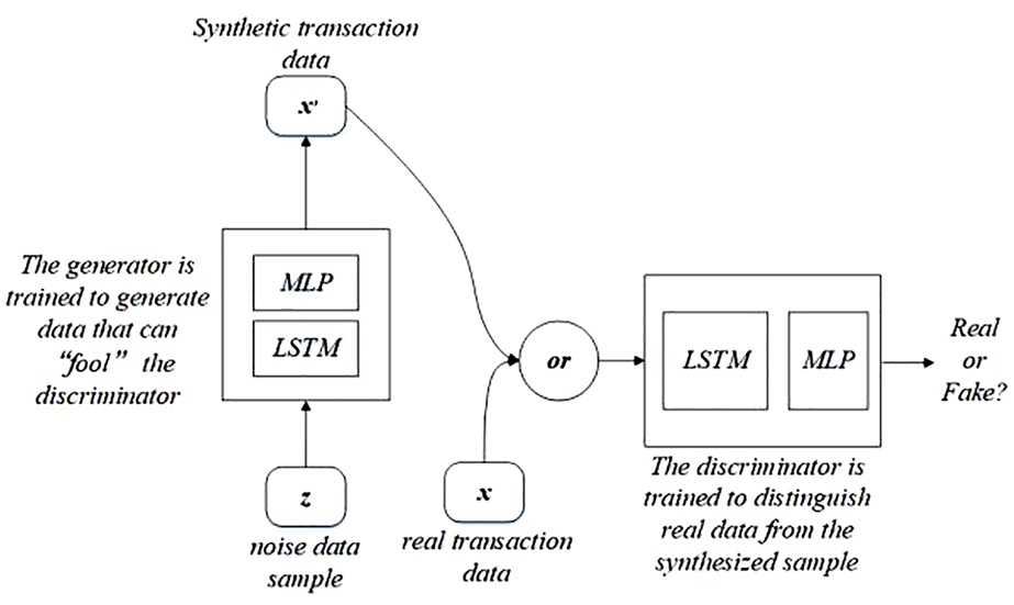
New generation model structure.
In proposed network structure, both generator and discriminator are based on LSTM network and MLP. The basic principle of generation model is consistent with the principle of the original GAN model, that is, the min-max game between

The detailed structure of generator.
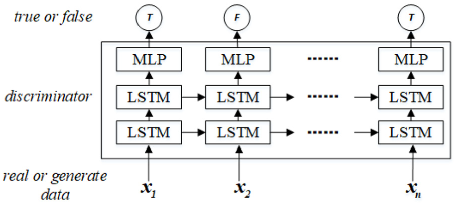
The detailed structure of discriminator.
Generation model
Figure 3 indicates that LSTM layer connects with the input layer and MLP layer. The generator first samples m noises

where
Moreover, after MLP layer, it maps hidden states


where
Discrimination model
In Figure 4, LSTM cells model the input features, maps them to hidden state, and finally distinguishes input data labeled 0 and 1 through neural networks.
For the input samples, we represent an input sequence


where
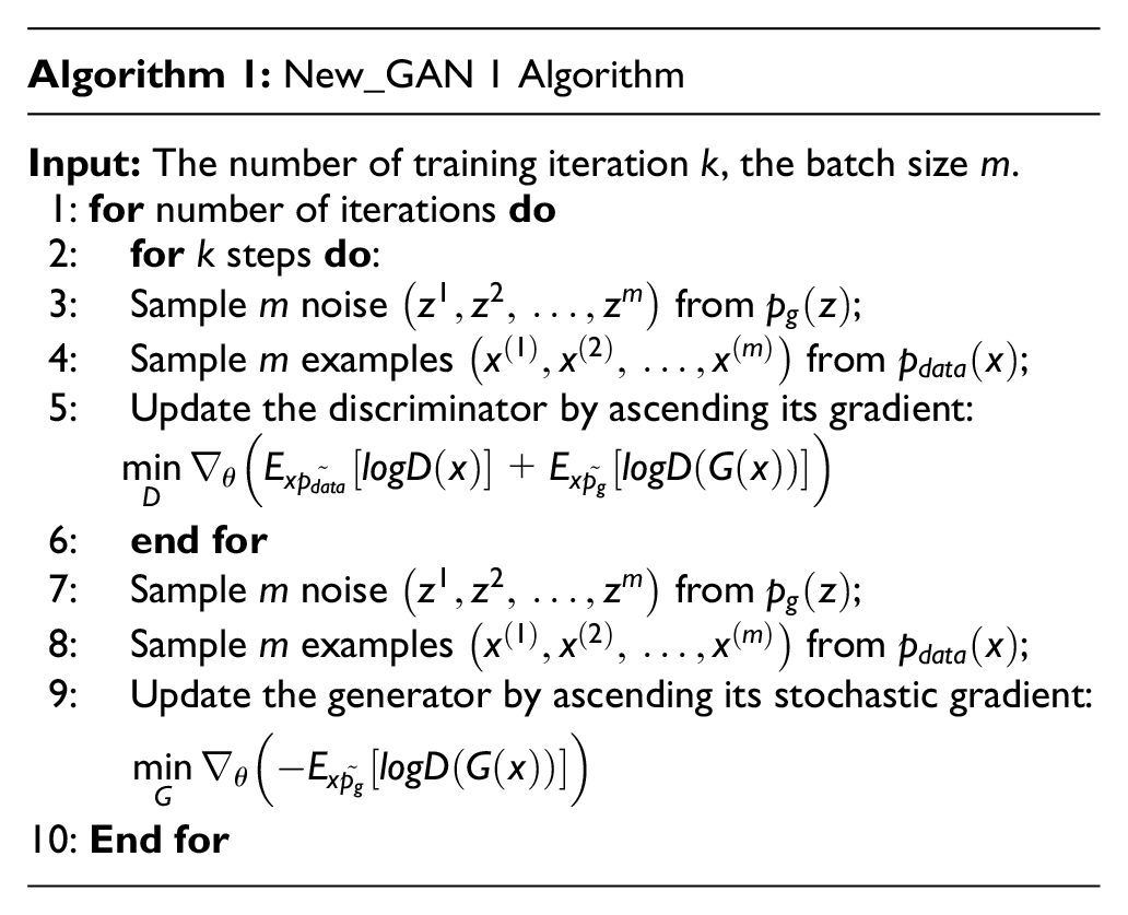
The optimization target is to minimize the objective functions between truth label and predicted probability. We adopt the adversarial training of generators and discriminators, and use the
The proposed algorithm is presented in Algorithm 1.
Update objective function
A persisting challenge in the training of GANs is model collapse. For example, we train GAN model with MNIST dataset. The trained GAN can only generate one of 10 numbers; or in experiment of the face image, only one style of image is generated. Arjovsky et al. 7 points out that the divergences which GANs typically minimize are not continuous and differentiable everywhere. While updating generator’s parameters, it leads to training difficulty. WGAN improves traditional GAN by using earth mover’s distance or Wasserstein distance. The definition of Wasserstein distance is
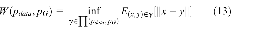
where
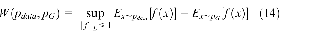
The supremum is 1-Lipschitz function

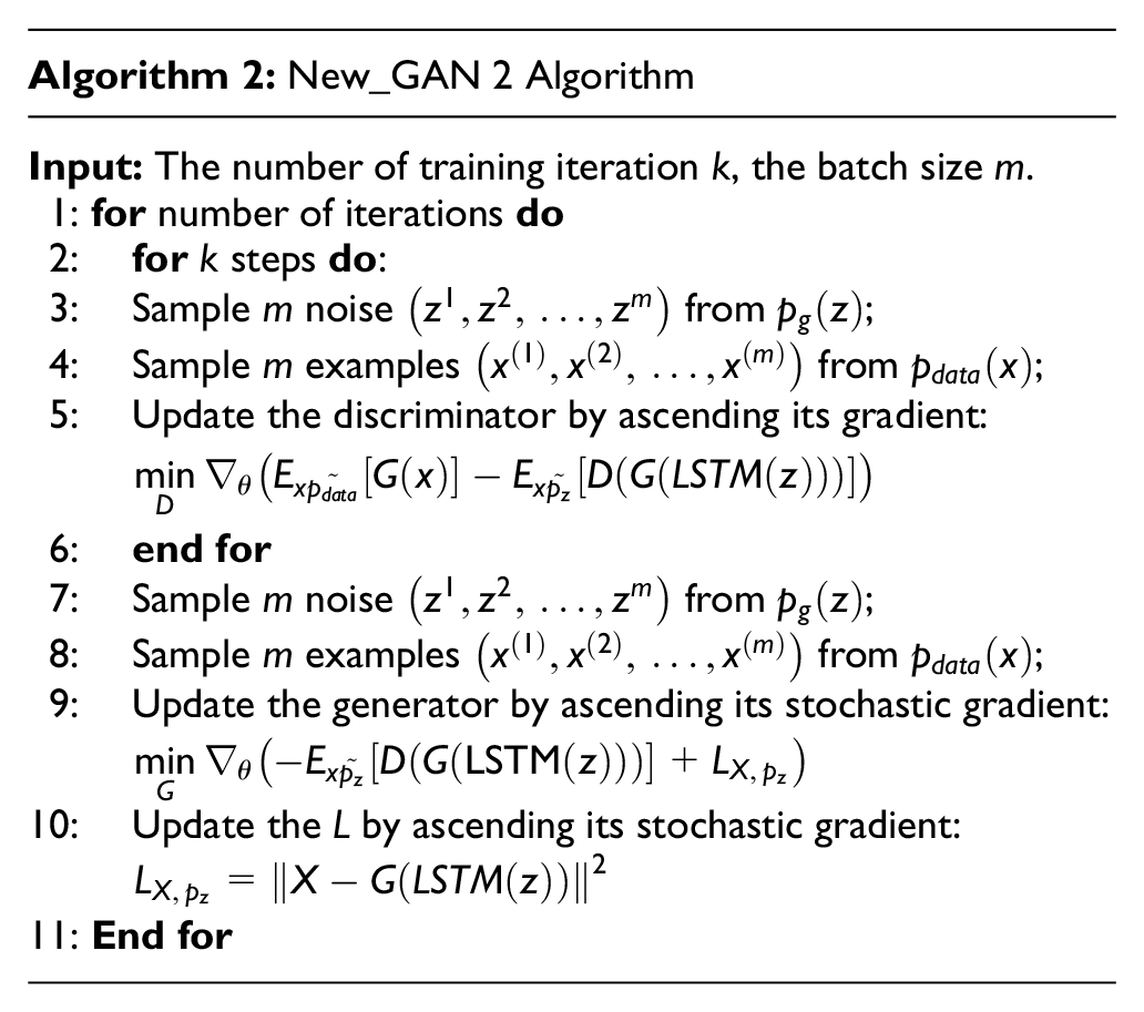
We use LSTM to capture useful local features and generate samples. The optimization target can be described as

After adding the feature matching penalty into generator, the optimized object of generator is to minimize

As for discriminator, it should get high confidence and

The proposed algorithm is presented in Algorithm 2.
Evaluation
In the “New Generation Model” section, the target optimization function of the proposed GAN model is log-likelihood function. However, log-likelihood estimation is difficult to process and measure whether our model well-trained or not. At present, the evaluation methods for GAN are example-based, which extract features from generated samples and real samples and then performs distance measurement in feature space. 24 The simple evaluation from the perspective of data distribution is not comprehensive, which ignores attribute characteristics of one-dimensional data. This article combines data distributions and data correlations to evaluate generated data for evaluating our generated samples comprehensively. Finally, we perform our generation samples with raw dataset on a binary classifier. The evaluation indexes indicate the quality of generation data.
Data distribution
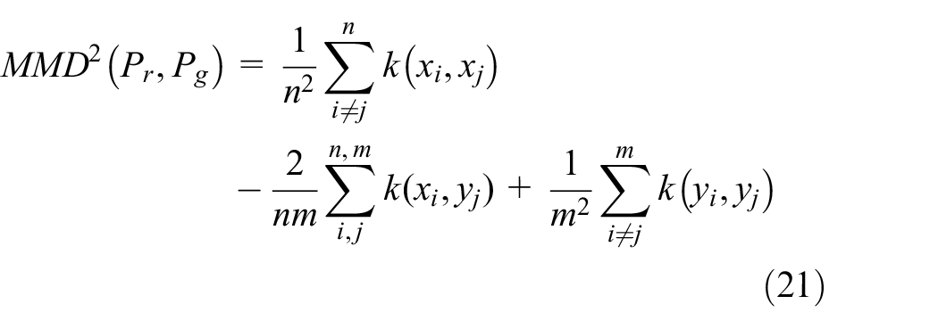
After training, assume that a successful GAN network can learn the true sample data distribution. The data distribution mapped onto feature space should also be same. We use Kernel MMD 6 method to calculate data feature distribution.
MMD is maximum mean discrepancy. Based on the samples of the two distributions
Suppose that the original dataset is

MMD launched as

Expanding formula, the form of
Since Gaussian kernel can be mapped to infinite dimensional space, and one-dimensional transaction data often has 10 to dozens of data attributes, the Gaussian kernel function

which means the smaller of the
Therefore, objective function of distribution measure can be written as

Feature correlations
Different from pictures, voice, and text data, there are strong correlations between different attributes in one-dimensional transactions. For example, when trading time is happened on 10:00 am, fraudulent transactions frequently occur in East China. It means that trading time and trading location are related. Therefore, we evaluate whether generated data attributes have same correlation with original data attributes.
Each transaction data can be expressed as

Mean
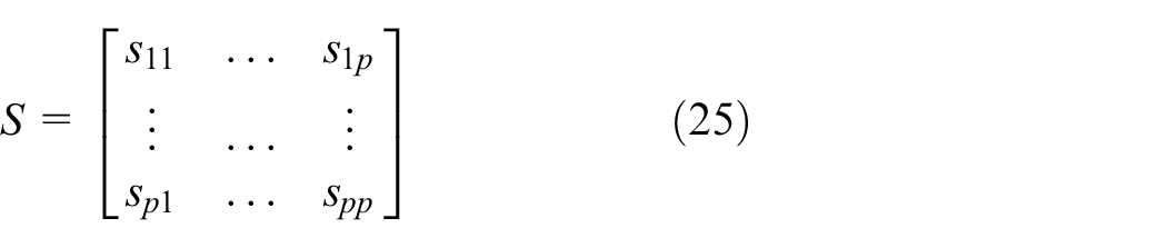
The correlation coefficient of attributes
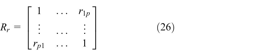
Similarly, for generated sample data

If the attributes

As correlation coefficient matrix is a symmetric matrix. Obviously, the smaller the

Comprehensive evaluation
According to two evaluation methods mentioned above, final evaluation function
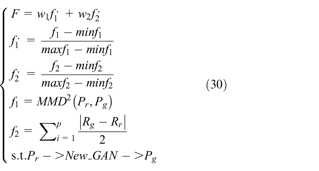
Among them,
When using the comprehensive evaluation indicator, multiple generation models compare the experimental calculation results. The smaller the indicator of the model, the better the generation effect and closer to the original distribution.
Experiment and evaluation
Experiment setup
Dataset description
The experiment data are from real online transaction data of a major domestic bank. Raw dataset contains 3 months of bank B2C transaction records, about 3-million transaction data, of which about 100,000 negative transactions. It is found that data characteristics such as transaction time and transaction amount can reflect user’s transaction behavior characteristics. We select eight-dimensional feature used as the sample data to input. As the data cannot be public, the selected data dimension is not able to describe in detail. To ensure data consistency and availability, the data are processed routinely, including data cleaning, data conversion, and data reduction.
Parameter settings
For discriminators and generators, we use LSTM cells and multi-layer fully connected networks. The LSTM layer is two layers, which is more conducive to remembering information; and there are two layers of fully connected layers. Since original data to be generated are eight-dimensional data, output layer of generator is eight nodes, and the same as discriminator’s input. The final layer of the discriminator doesn’t contain any non-linear activation function. We use backpropagation algorithms to track learning conditions and adjust network parameters. Following the proposed method, we train the generation model for 100 epochs, saving one version of the dataset every 10 epochs and records MMD value every epoch.
Model training
Training with MMD
As we can reach data distribution, model records MMD’s value after each epoch during the model training, as shown in Figure 5.

MMD value with every epoch.
Figure 5 shows that as training epoch increases, MMD value between generated samples and real samples remain smoothly, below 0.002.
We can see generated sample distribution is completely similar to real sample distribution. The generator could generate “real” data. It is encouraging to observe that the likelihood of the generated samples improves with training.
Training result
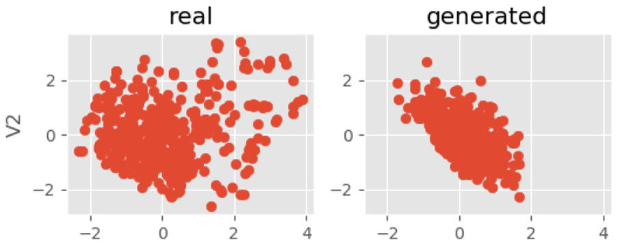
After training, we record the visual results of each training. Figures 6–8 are two-dimensional visualization pictures of v1 and attribute v2 in the data attribute after training, where the y-axis is v2 and the x-axis is v1. Figures 9–11 are two-dimensional visualization pictures of v3 and attribute v1 in the data attribute after training, where the y-axis is v3 and the x-axis is v1. The pictures of the training are shown in the figure below.
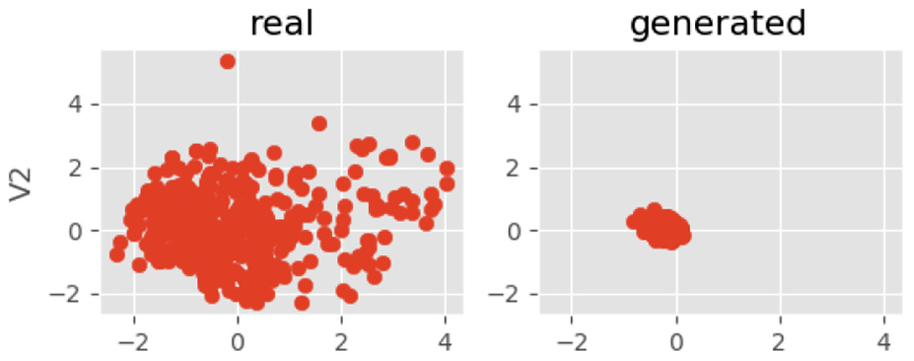
V2 epoch = 10.
V2 epoch = 50.
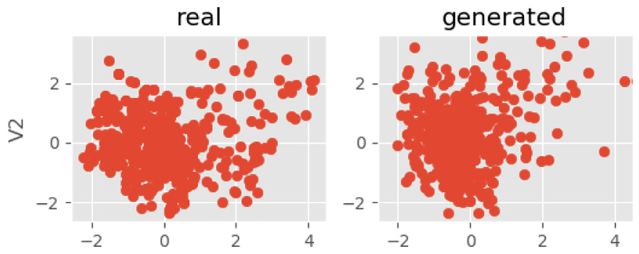
V2 epoch = 100.

V3 epoch = 10.

V3 epoch = 50.

V3 epoch = 100.
The left side of the picture is the distribution of real input data, and the right side is the case of generating data. It can be seen from the figures that as the number of training increases, the generated data are getting closer to real data distribution. It can be explained that our model is well trained. The generator captured raw data distribution.
Model verification
Comprehensive evaluation
The weights are divided into two principles; each is set to 0.5. For trained model, different numbers of data are generated, and the score of comprehensive evaluation method is calculated. The baseline model is regular GAN 3 and VAE. 4 We train the proposed model and baseline model. After model well trained, we generate different test subsets and calculate each dataset’s comprehensive score. The comprehensive evaluation score is shown in Table 1.
Comprehensive evaluation score.

GAN: generative adversarial network; VAE: variational autoencoder.
Bold numbers indicate the optimal experimental results for each dataset.
It shows that calculated values of our two model under comprehensive evaluation are all below 0.2. Generated data are close to original data distribution. In D_s3, the value is below 0.1 and the quality of the generated data is excellent. Then, we introduces Wasserstein distance and penalty into New_GAN2. It can be seen that the score is lower than New_GAN1 in D_s4 and D_s5. Compared with New_GAN1, the score of D_s4 has decreased by 10% and D_s5 has dropped about 20%. The New_GAN2 can completely approximate real data, and the generation data are more controllable and realistic.
To further validate the model classification results, we use a classification model to verify and the experimental results are described in next section.
GAN classify
We perform our model on classification model. The generated data are added to raw dataset to constitute a newly dataset. The quality of the generated data is tested by a binary classifier on multiple synthetic datasets. The basic evaluation index is accuracy, precision, and recall. The confusion matrix is shown in Table 2.
The confusion matrix.

Accuracy is the ratio of correctly classified by the classifier to total numbers of samples
Precision is the ratio of positive samples that are classified correctly to number of samples that classifier determines to be positive samples:
Recall is the ratio of positive samples with correct classifications to true positive samples:
In the GAN generated data1, VAE generated data2, New_GAN1 generated data3, and New_GAN2 generated data4, the model classification effect is compared. The results of this experiment are presented in Figures 12–14, which compares the performance achieved by the classifier.

The classify performances of models on Dataset1.
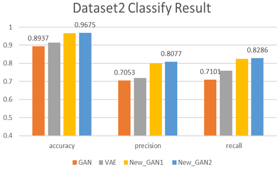
The classify performances of models on Dataset2.
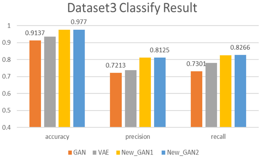
The classify performances of models on Dataset3.
As the figure room is not sufficient. Thus, we just list the data label in the max and min dataset. It can be seen from figures that generating data improve the original model classification effect. Among them, our generation models, compared with baseline models: GAN and VAE, have the advantage of enhancing data in generating negative transaction data. Our model has achieved best detections on all three test subsets. In terms of accuracy, classification results of the datasets generated by New_GAN1 and New_GAN2 models are above 95%, the accuracy is above 70%, and the recall rate is about 83%. Compared with VAE and original GAN, the classification results of the two models proposed in three datasets are improved about 5%, the accuracy is improved by about 8%, and the recall rate is up to 10%. The accuracy and recall of New_GAN model increased by average of 5%. However, with New_GAN1, the results of New_GAN2 on three datasets of evaluation metrics are not significantly improved. It has a certain relationship with the upper limit of the classification model itself.
Compared with other two baseline models, the generative model with LSTM networks proposed in this article is good at enhancing data classification results. The model we proposed in this article is superior to the existing GAN model and the VAE model in the effect of generation real samples. And the generation model New_GAN2 based on Wasserstein distance and penalty is better than New_GAN1.
Conclusion
Through our work, it can be found that the combination of GAN and LSTM network has achieved excellent performance. GAN network is suitable to quickly capture the characteristics of data distribution. LSTM can generate data with time series, which retains data distribution of generated data. Our work provides a novel method to generate “realistic” data in financial transaction data to naturally solve imbalanced problem. For the generated one-dimensional sample data, we evaluate the quality of the generated data from three aspects: data distribution, data attributes, and classification effects.
Although our generation model achieves better improvements in results, we have encountered a lot of difficulties while model training. From the model perspective, generators and discriminators need to be carefully balanced. And the generator is easy to fall into the local optimum, resulting in a single sample and insufficient diversity. In the future, we will improve the model from the perspective of loss function, gradient penalty, and so on. And our GAN can generate data similar to the real data, and cannot generate the potential fraud that has not yet occurred under the data latent space. The diversity of generated samples is insufficient, and it is difficult to cope well with potential cases that have not occurred. From this perspective, we will better solve the negative sample problem in financial transactions.
Footnotes
Handling Editor: Liran Ma
Declaration of conflicting interests
The author(s) declared no potential conflicts of interest with respect to the research, authorship, and/or publication of this article.
Funding
The author(s) disclosed receipt of the following financial support for the research, authorship, and/or publication of this article: This work was supported by Natural Science Foundation of Shanghai (No. 19ZR1401900), Shanghai Science and Technology Innovation Action Plan Project (No. 19511101802), and National Natural Science Foundation of China (No. 61472004, 61602109).