
Abstract
A large number of smart devices make the Internet of Things world smarter. However, currently cloud computing cannot satisfy real-time requirements and fog computing is a promising technique for real-time processing. Operational modal analysis obtains modal parameters that reflect the dynamic properties of the structure from the vibration response signals. In Internet of Things, the operational modal analysis method can be embedded in the smart devices to achieve structural health monitoring and fault detection. In this article, a four-layer framework for combining fog computing and operational modal analysis in Internet of Things is designed. This four-layer framework introduces fog computing to solve tasks that cloud computing cannot handle in real time. Moreover, to reduce the time and space complexity of the operational modal analysis algorithm and support the real-time performance of fog computing, a limited memory eigenvector recursive principal component analysis–based operational modal analysis approach is proposed. In addition, by examining the cumulative percent variance of principal component analysis, this article explains the reasons behind the identified modal order exchange. Finally, the time-varying operational modal identification results from non-stationary random response signals of a cantilever beam whose density changes slowly indicate that the limited memory eigenvector recursive principal component analysis–based operational modal analysis method requires less memory and runtime and has higher stability and identification effect.
Keywords
Introduction
In Internet of Things (IoT), enormous sensors and smart devices are embedded in hospitals, railways, bridges, tunnels, roads, buildings, dams, and other objects to collect data, allowing the connection between objects. However, these data should be processed and mined further to obtain implicit information. Operational modal analysis (OMA) aims to extract modal ratios, natural frequencies, and modal shapes, called modal parameters, from vibration sensors. 1 Recently, OMA has become an effective tool for large structures, because it does not need to measure inputs that are usually unavailable. The application of OMA in the Internet of Things has fault diagnosis, structural health monitoring, and so on. 2
Since the actual mechanical structure is usually linear time-varying (LTV), its stiffness, mass, damping, or temperature will change with time. For example, the vehicle–bridge vibration structure is a variable mass time-varying structure. 3 In addition, in real life, data are obtained one after another. Therefore, the data processing method should be online and in real time and can adapt to time-varying or non-stationary characteristics. 4
Recently, time domain approaches and (time) frequency domain methods are the main OMA algorithms for LTV structures. 1 Time domain methods are more widely studied and can be divided into time-dependent state space (TSS)-based and time series–based methods. Liu and Deng 5 developed a new TSS method that is less sensitive to noise and verified using moving cantilever beam. Ma et al. 6 proposed a parametric LTV method using kernel recursive extended least squares time-dependent autoregressive moving average. Their algorithm achieves O(N2) time and space complexity. As for the frequency domain approaches, Dziedziech et al. 7 presented a wavelet-based method for LTV structure, which uses random impact excitation to obtain the frequency response function. The above methods can identify the modal parameters for LTV structure, but they are offline or batch-wise. Wang and colleagues 8 used moving window and proposed a limited memory principal component analysis (LMPCA)-based OMA approach to make principal component analysis (PCA)-based method suitable for slow LTV structures. After that, Wang et al. 9 presented a limited memory recursive principal component analysis (LMRPCA)-based OMA approach to reduce time and space complexity. In summary, in order to apply these methods to online fault diagnosis and structural monitoring, it is necessary to further reduce the complexity of these algorithms.
Cloud computing improves the capabilities and application scenarios of IoT.10,11 In IoT, the sensor networks are used to collect data12–14 and cloud computing provides storage and computing capabilities to ease the burden on sensors.15,16 However, it takes time to transfer data to the cloud and receive feedback from the cloud. Compared with cloud computing, fog computing is a promising technique for IoT. 17 Serving as a link between sensor networks and the cloud, the fog can process and store data near where they are produced and then manage and control sensors at a short distance. The fog computing is also called edge computing. 18 Recently, there are many challenges on fog computing and IoT, such as trust evaluation,19,20 security,21,22 resource allocation,23–25 and privacy.26,27 Wang et al. 28 proposed a fog-based hierarchical trust mechanism to solve cyber security problem and the data analysis task is conducted in fog layer. Li et al. 29 developed a framework for indoor localization technology under mobile edge computing environment. Wang et al. 30 proposed a novel framework that makes it possible to assign some storage and computing tasks to the fog servers and ensure data privacy. The data upload problem in fog computing is simplified from a graph theory perspective into a combinatorial optimization problem. 31 Wang et al. 32 proposed a new framework that reduce resource consumption and improve the efficiency of IoT devices. Yin and Wei 33 constructed a communication-efficient data aggregation tree for complex queries in IoT applications, which reduces communication cost. The development of smart devices has enabled the collection of more valid data. Big data, which contain a lot of useful information, and IoT contribute to the development of the smart cities.34–36 Fog computing is used to assist cloud computing in processing data, especially tasks that require real-time processing. 37 Coincidentally, OMA for LTV structures aims to needs to process the data obtained in succession in real time. Thus, it is feasible to combine fog computing with OMA.
To reduce the time and space complexity of the algorithm, a limited memory eigenvector recursive principal component analysis (LMERPCA)-based approach is designed. This OMA method uses a rank 1 matrix for eigenvector recursion to identify modal parameters for LTV structure and achieves the time and space complexity of O(N). 38 An earlier version combined LMERPCA with cloud computing and was presented at the SCS2019 conference. 39 This article designs a new architecture to combine LMERPCA with fog computing. Furthermore, we add an explanation and the simulation verification for the reasons of modal exchange. In the simulation section, we add a comparison of this method to the state of the art. The experimental results and analysis have also increased.
In summary, our contributions are fourfold:
We combine ERPCA and moving window and propose LMERPCA-based OMA method to extract the transient modal shapes and natural frequencies. We also propose a framework to combine fog computing with LMERPCA-based OMA.
LMERPCA-based OMA offers a faster runtime and lower memory consumption. Since this method directly obtains the modal shapes and modal responses through a recursive method, it can achieve higher recognition accuracy.
We compute the change in the cumulative percent variance (CPV) for slow linear time-varying structure (SLTV) and explain the reasons for modal exchange in LMPCA- and LMRPCA-based OMA in such structures.
We design a variable density cantilever beam simulation to verify the performance of LMERPCA-based OMA.
The remainder of this article is structured as follows. The LMERPCA-based operational modal online identification for SLTV structures is then described in section “Combining LMERPCA-based OMA with Fog Computing in IoT,” and simulation results are analyzed and compared in section “Simulation.” In the last section, we conclude this article.
Combining LMERPCA-based OMA with fog computing in IoT
Vibration representation of slow LTV structure based on time-freezing theory
In time-varying structures, the vibration response also changes with time. According to structural dynamics theory, the dynamic equation in the physical coordinate system is expressed as follows
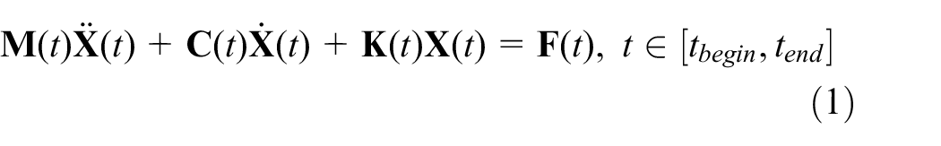
where
Non-stationary response signals decomposition in modal coordinate for SLTV
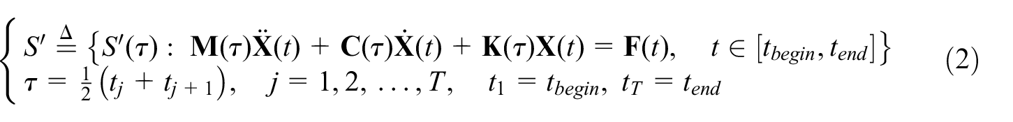
Based on the “time-freezing” theory, the frozen-in coefficient method, the “short-time invariant,” and “quasi-stationary” assumptions, the SLTV structures can be approximated as multiple linear time-invariant structures in short-time intervals. Every time interval is seen as a window. Figure 1 shows update process of fixed-length moving window.

The data window moves to the right.
The choice of moving window length is fixed (the length is

where
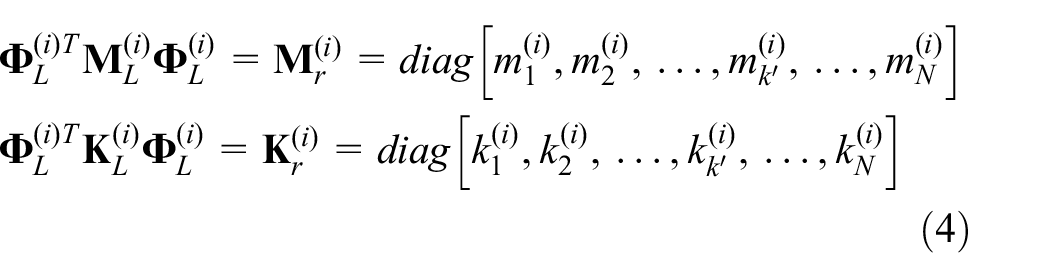

From equations (4) and (5), we can see that
The derivation of LMERPCA algorithm
Moving window is a limited memory method. During the moving window, new data
Set the window length as L. At time

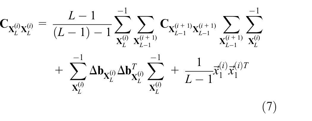
where
When adding a new data, the model is updated, so the overall variance and average gradually change. Therefore, equation (7) can be simplified using original model as

where
We orthogonally decompose

where

Setting

Modifying equation (4) as

we can further transform equation (11) into
Setting
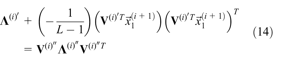
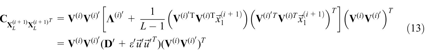
After applying rank 1 correction twice,
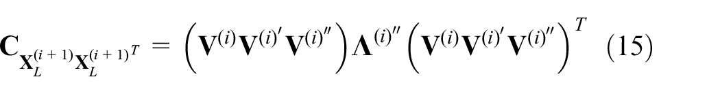
Finally,


The LMERPCA-based OMA algorithm for SLTV structures in IoT
After the eigenvectors and PCs are obtained by the LMERPCA algorithm, the modal parameters can be identified. That is, the modal shape can be obtained from the eigenvectors and the natural frequency can be calculated from the PCs. Figure 2 shows the entire identification process. The moving window method allows fixed-length data matrix to be identified at each moment. Table 1 compares the performance of LMPCA-, LMRPCA-, and LMERPCA-based OMA algorithms.
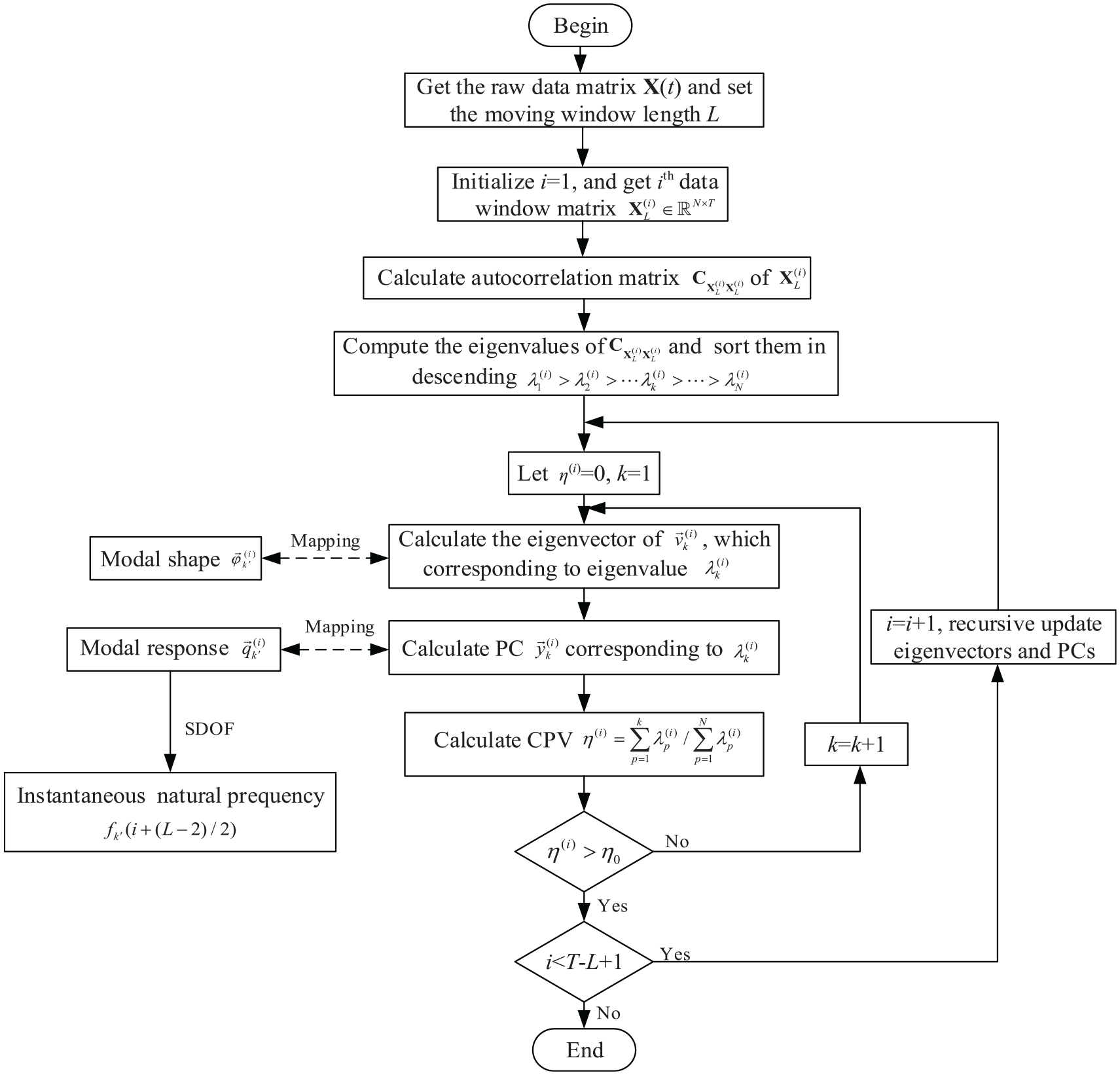
The modal parameter identification process of LMERPCA-based OMA approach.
Performance comparison of three modal parameter identification methods.

LMPCA: limited memory principal component analysis; OMA: operational modal analysis; LMRPCA: limited memory recursive principal component analysis; LMERPCA: limited memory eigenvector recursive principal component analysis.
Fog computing devices have certain computing and storage capabilities. However, these capabilities are limited. Our LMERPCA-based OMA algorithm is embedded into the fog computing devices to process data (identify modal parameters). Therefore, the memory occupied by the embedded algorithm should be as small as possible. Meanwhile, to support the online and real-time processing, the proposed method should have the ability to identify quickly. In short, to support fog computing, the proposed algorithm needs low time and space complexity.
CPV of PCA model and modal exchange in LMPCA- and LMRPCA-based OMA
The order of the mode identified by PCA depends on its contribution rather than its frequency value. 40 The greater the contribution, the faster the mode will be identified, and a Pareto chart can be constructed to show the contribution of each mode. The CPV is used to represent the proportion of PCs extracted in the PCA method. 40
For SLTV structures, the engineering damping, stiffness, and mass change over time resulting in a change in the order of each modal contribution rate. Due to the modal change, the frequency order of recognition is inconsistent with the order of contribution. The correspondence between the two order rankings may also change over time. For example, assuming the CPV
In LMPCA- and LMRPCA-based OMA for SLTV structures, the eigenvectors and PCs are calculated by eigen value decomposition (EVD) or singular value decomposition (SVD) of the autocorrelation matrix and re-ordered according to descending eigenvalues. With changes in the CPV of each modal at every data window, the identified modal order may change in some data windows. However, in LMERPCA-based OMA, rather than applying EVD or SVD to the autocorrelation matrix and re-ordering according to the eigenvalues, we simply calculate the PCs and eigenvectors using SVD or EVD in the first data window and update the PCs and eigenvectors in other data windows recursively without re-ordering them. Hence, changes in the identified modal order can never occur in LMERPCA-based OMA approach.
Framework for combining fog computing with LMERPCA-based OMA in IoT
In IoT, the displacement, acceleration, or velocity vibration sensors are embedded in various SLTV structures (bridges, buildings, vehicles, etc.). The vibration sensor can obtain non-stationary random vibration response signals of the SLTV structure under ambient or working excitation. Then, LMERPCA-based adaptive operational modal real-time identification method can be used to extract the time-varying structural dynamics information from these non-stationary random vibration response signals. Therefore, LMERPCA-based OMA method enables structural dynamic design and fault diagnosis in IoT.
Our framework includes four layers: (1) wireless sensor network layer: used to collect the non-stationary random vibration response signals; (2) fog layer: used to process the LMERPCA-based adaptive operational modal identification real-time tasks; (3) cloud layer: used to call the relevant data from the sensor network layer and process non-real-time tasks; and (4) user layer: refer to the user who needs a service or request such as structure online health monitoring or vibration control. The fog layer handles the tasks that are processed in real time and relatively few computations. If the task request received by this cloud layer is real time, the cloud layer assigns the task to the fog layer. If the task received by the fog layer is not real time, it is passed to the cloud layer.
In theory, the greater the number of vibration sensors, the more accurate the modal parameters identified. However, the number of vibration sensors is limited in actual engineering. Vibration sensors should be arranged in the locations that primarily reflect the vibration mode of the structure. The LMERPCA algorithm requires that the number of vibration sensors is greater than or equal to the number of identifiable modes. Fog computing is proposed to enable computing directly at the edge of sensor networks and the fog devices have some local computation and storage capacity. In other word, the data can be quickly transferred to the fog layer. Fog computing greatly reduces the amount of time that data are transferred to the cloud. Without fog computing, the data should be transmitted to the cloud layer and cannot process in real time. This framework of combining fog computing with LMERPCA-based OMA in IoT is shown in Figure 3.

The framework of combining fog computing with LMERPCA-based OMA in IoT.
Simulation
Parameters of SLTV cantilever beam
A cantilever beam model
8
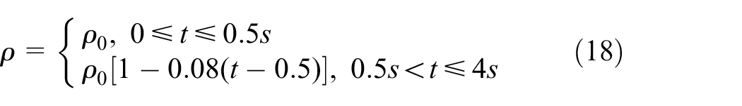
with dimensions of 1 m × 0.02 m × 0.02 m (length × height × width), cross-sectional area A = W × H = 4 × 10⁻⁴ m2, density
The total simulation time is 4 s. Figure 4 shows the time-varying transient natural frequencies of the first 10-order mode of the start and end times.

Change in transient natural frequencies (0–4 s).
Simulation parameters setting
In this simulation, we used the Newmark-β approach to obtain the displacement response signals of virtual displacement sensors. The proportional coefficients were set to βM = 4 × 10⁻⁴ and βK = 1 × 10⁻⁷. The initial displacement and speed were set to zero. According to sampling theory, the sampling frequency was set to 10,000 Hz, and the integration step size of Newmark-β was set to 1/10,000 s. 39 The window length L was set to 4096 9 and the parameter η0 in Figure 2 was set to 95%. In the time domain, 2.0% Gaussian measurement noise was added to the displacement response signals. The noise was

where r is the noise level and e is a normal random vector with a standard deviation of 1 and an average of 0. The test system parameters are the same as those used in Guan et al. 8 and Wang et al., 39 and the purpose is to obtain simulated vibration response signals. These signals are measured by vibration sensors in practice.
Experimental quantitative evaluation index
To evaluate the recognition accuracy of the modal shape, the modal assurance criterion (MAC) which value ranges from 0 to 1 is used. The MAC 40 is defined as

where
Transient operational modal parameter identification results
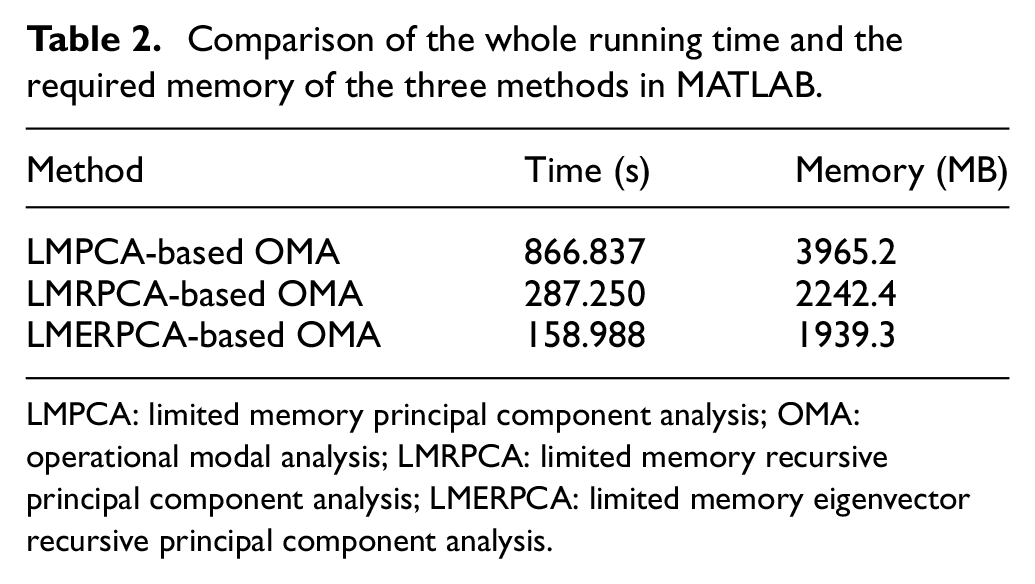
The fourth subfigure of Figure 5(a) and (b) is the Pareto charts, indicating the ratio of the extracted PCs. The theoretical values were calculated from the analytical solution. We randomly selected two moments, 1.7028 and 2.2547 s. Figure 5 shows the modal shape identification results of three OMA methods at two moments. Figures 6 illustrates the results of the first three orders of frequency identification for the three OMA methods. The quantified results of the first three orders of modal shape identification are shown in Figure 7. Table 2 compares the running time and memory of the three methods in MATLAB 2016b for all windows. Figure 8 is a variance contribution rate of the third- and fourth-order modes.
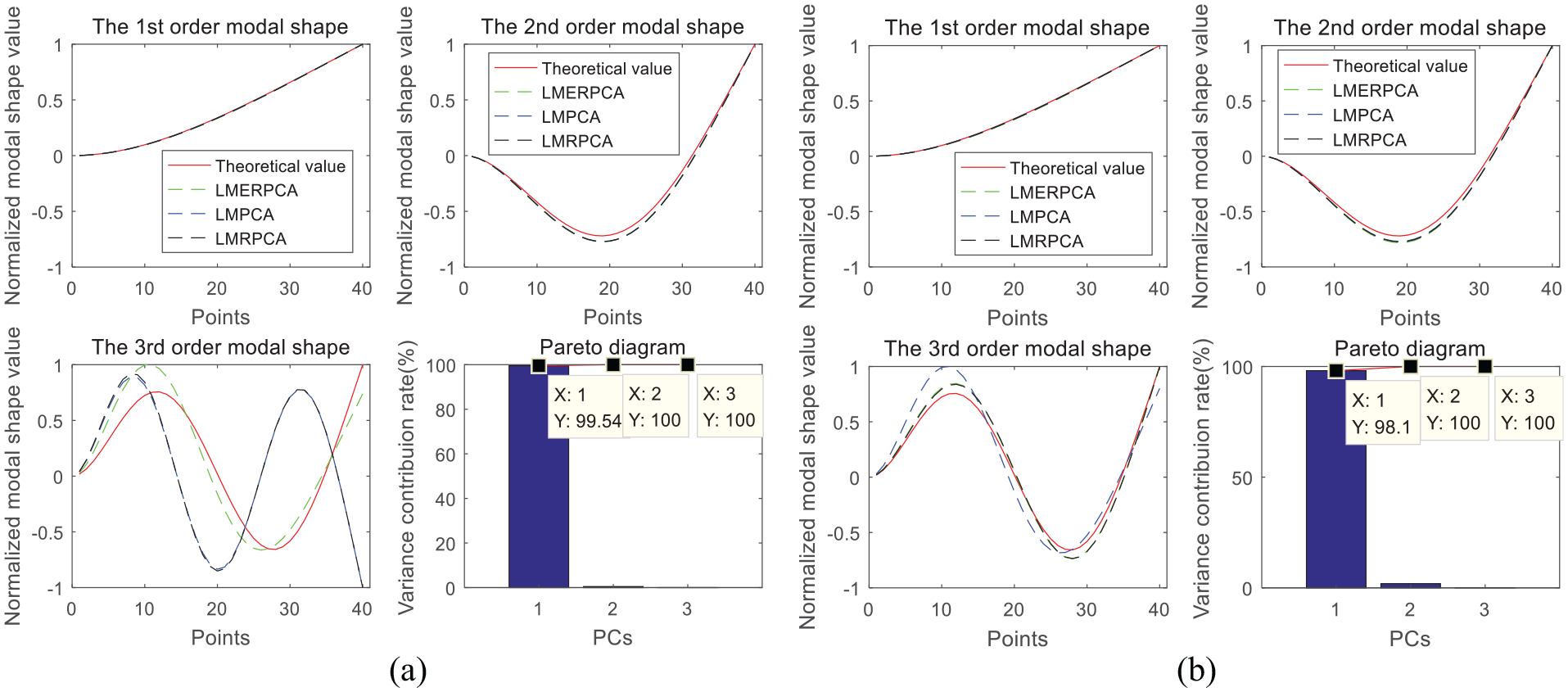
Comparison of transient modal shape results identified by LMPCA, LMRPCA, and LMERPCA: (a) in 1.7028 s and (b) in 2.2547 s.

Comparison of frequency results identified by LMPCA, LMRPCA, and LMERPCA: (a) first PC, (b) second PC, and (c) third PC.

MAC values recognized by LMPCA, LMRPCA, and LMEPCA.
Comparison of the whole running time and the required memory of the three methods in MATLAB.
LMPCA: limited memory principal component analysis; OMA: operational modal analysis; LMRPCA: limited memory recursive principal component analysis; LMERPCA: limited memory eigenvector recursive principal component analysis.

Variance contribution rate of the third- and fourth-order modes.
Analysis of operational modal identification results
Figures 5–7 indicate that the LMERPCA-based OMA method can well identify the modal shapes and natural frequencies of a cantilever beam with a slow time-varying density. It also shows that the LMERPCA-based OMA method is not sensitive to noise.
The Pareto charts in Figure 5(a) and (b) show that the first three orders of CPV reach 99.999%, that is, the entire vibration characteristic can be represented by the third order.
According to the comparison of LMPCA, LMRPCA, LMERPCA, and the theoretical values in Figure 6, the frequencies identified by LMERPCA-based OMA form a ladder shape. The reason for this shape in the identified transient frequencies is that the FFT is 2.44 Hz, and the frequency variations
The order of the mode identified by PCA depends on its contribution, rather than its frequency value. At some point between 1.68 and 1.89 s, Figure 6(c) shows that the third frequency identified by LMPCA- or LMRPCA-based OMA is the same as the fourth theoretical natural frequency. Figure 8 shows the contribution to the variance of the third- and fourth-order modes. Most of the time, the variance contribution of the third-order mode is greater than that of the fourth order. Comparing Figure 5(a) and (b), the order of the identified modes has changed. In Figure 5(a), the third theoretical modal shape corresponds to the fourth identified modal shape. Figures 5, 6, and 8 reveal that there is no modal exchange in the proposed LMERPCA method, while there is a modal exchange in LMPCA and LMRPCA. Therefore, the LMERPCA method has better accuracy and the order of the identified modes remains stable.
Table 2 shows that LMERPCA-based OMA has the least runtime and memory because LMERPCA obtains PCs and eigenvectors by eigenvalue eigenvector recursive rather than autocorrelation matrix recursive. This is the total time and memory of more than 30,000 data windows, and the time and memory requirements of each data window are very small. Therefore, LMERPCA-based OMA approach can be more suitable for integration into fog server devices and can be used in structural health monitoring in IoT.
Conclusion
This article proposed an adaptive operational modal real-time identification in fog computing–based IoT. LMERPCA-based OMA approach has low time and space complexity and can well identify the modal parameters of slow LTV structure in noise. Then, we design a four-layer framework for integrating this OMA method and fog computing to meet real-time requirement of users. Furthermore, by examining the CPV of PCA, this article explains the reasons behind the identified modal order exchange.
However, the recognition result of the moving window is the result of the time corresponding to the intermediate data, so the values of some moments are not recognized. The adaptive selection of moving window length further reduce the complexity of time and space, and the comparison of the cloud computing and cloud-fog synergy methods and the application of methods to more complex LTV structures are further research directions.
Footnotes
Handling Editor: Xiaoyang Wang
Declaration of conflicting interests
The author(s) declared no potential conflicts of interest with respect to the research, authorship, and/or publication of this article.
Funding
The author(s) disclosed receipt of the following financial support for the research, authorship, and/or publication of this article: This work has been financially supported by the National Natural Science Foundation of China (Nos 51305142, 51305143, 18BTJ031, and 71571056), the Postgraduate Scientific Research Innovation Ability Training Plan Funding Projects of Huaqiao University (No. 17013083018), the Quanzhou Science and the Technology Plan (No. 2018C110R), and the National Science Foundation (No. DMS-0907710).