
Abstract
Recently, as demand for high-quality video and realistic media has increased, High Efficiency Video Coding has been standardized. However, High Efficiency Video Coding requires heavy cost in terms of computational complexity to achieve high coding efficiency, which causes problems in fast coding processing and real-time processing. In particular, High Efficiency Video Coding inter-coding has heavy computational complexity, and the High Efficiency Video Coding inter prediction uses reference pictures to improve coding efficiency. The reference pictures are typically signaled in two independent lists according to the display order, to be used for forward and backward prediction. If an event occurs in the input video, such as a scene change, the inter prediction performs unnecessary computations. Therefore, the reference picture list should be reconfigured to improve the inter prediction performance and reduce computational complexity. To address this problem, this article proposes a method to reduce computational complexity for fast High Efficiency Video Coding encoding using information such as scene changes obtained from the input video through preprocessing. Furthermore, reference picture lists are reconstructed by sorting the reference pictures by similarity to the current coded picture using Angular Second Moment, Contrast, Entropy, and Correlation, which are image texture parameters from the input video. Simulations are used to show that both the encoding time and coding efficiency could be improved simultaneously by applying the proposed algorithms.
Keywords
Introduction
In the past several years, the development of high-speed communication lines and multimedia technology have enabled mass adoption of diverse multimedia contents service, and the requirement and expectation of users for high definition video service and immersive media are continuously increasing. Various high-definition (HD) video services through the Internet are provided not only for PCs but also for various portable terminal devices such as smart phones and tablets. With the development of Me-Media, a variety of types of content is being created through Me-Media broadcasting beyond texts and pictures. Furthermore, with the development of smartphone cameras and video equipment, individuals can now enjoy ultrahigh definition (UHD) broadcasting as well as HD broadcasting. Moreover, in order to enjoy immersive media, demand for virtual reality (VR), augmented reality (AR), mixed reality (MR), as well as super resolution and four-dimensional (4D) content is increasing. As users’ requirement for realistic media increases, the color space that expresses the color of the video is widened with the increase in the resolution, so that videos are displayed with colors more similar to the colors of natural objects, thereby enhancing the immersive feeling of users. There are user demand videos with high resolution, wide color gamut, high frame rate, and high bit depth, which contain much higher volume of data than existing videos. As the demand for such high-resolution content is expected to surge faster than the spread of the network infrastructure to transmit the content, a compression standard for ultrahigh-resolution content has been required. 1 ISO/IEC MPEG and ITU-T VCEG have formed the Joint Collaborative Team on Video Coding (JCT-VC) with the goal of achieving twice the compression ratio of H.264/AVC. 2 Under this goal, High Efficiency Video Coding (HEVC) version 1 was completed at the Geneva Conference in Switzerland in January 2013. 3 Compared with the conventional H.264/AVC, HEVC has standardized high-resolution video compression and high-speed parallel processing as main issues while keeping the overall encoding/decoding architecture similar. HEVC uses three types of temporal predictions: all intra (AI), low delay (LD), and random access (RA). In addition to the temporal prediction structure, HEVC employs the same spatial-temporal prediction, transformation, quantization, and entropy coding procedure as the existing video codecs like MPEG-2/4 and H.264/AVC, which compress the video based on hybrid video coding. Instead of the macro block unit used in H.264/AVC, the quad-tree structured coding unit (CU), prediction unit (PU), and transform unit (TU) are adopted in HEVC. Also, HEVC has various transform methods, using discrete cosine transform (DCT) and discrete sine transform (DST) in partial mode, prediction of improved motion vector with advanced motion vector prediction (AMVP) and merge mode, intra-prediction in 35 direction modes, in-loop filter function through deblocking filter and sample adaptive offset (SAO), entropy technology using CABAC, and so on. With these technologies, HEVC has a coding efficiency of approximately 40% or more in terms of objective video quality, which is equal to approximately 50% or more in terms of subjective video quality compared to H.264/AVC. 4 However, the techniques that achieve higher coding efficiency than H.264/AVC result in the high complexity of HEVC. In the research by Ahn et al., 5 when comparing the performance between JM 18.3 and HM 6.0 for bit rate and objective image quality, HEVC showed a bit rate reduction of 24.3%–44.2% over H.264/AVC. Although the encoding performance could be improved by various encoding schemes and the improved prediction method, the computational complexity is dramatically increased compared to H.264/AVC.6–8 Among the techniques used in HEVC encoding, inter prediction takes up to 89.1% of the total encoding complexity. In inter prediction, motion-compensated prediction using multiple reference pictures is used to improve coding efficiency, but has high computational complexity. 9 It is highly desirable to reduce the computational complexity of HEVC encoding while simultaneously maintaining the coding efficiency without significant degradation of visual quality. Various techniques and methods have been proposed and published in the literature to reduce the computational complexity of HEVC encoding.
Many types of video materials, such as movie trailers, music videos, and news, contain frequent scene cuts. Sometimes scene cuts are abrupt. Coding of a scene transition is often a challenging problem from the point of view of compression efficiency, because motion compensation (MC) may not be a powerful enough method to represent the changes between pictures in the transition. In this article, we propose a method of fast HEVC inter-coding that uses the scene-change information and texture features extracted from input video through preprocessing. Inter prediction is a prediction method using temporal redundancy in a video. HEVC reference software composes group of pictures (GOP) by dividing it into constant intervals, and the reference picture list (RPL) for inter prediction is composed using the coded pictures in the GOP. However, this approach does not consider information about the scene such as scene changes, but divides it into a certain size, thereby making unnecessary prediction calculation for a picture without temporal redundancy. To further improve the conventional approach, we propose a new method of reconstructing the RPL by advanced detection of an event contained in the input video. And, we propose an extended method of reconstructing the RPL by sorting the reference pictures in the order of similarity to the current coded pictures using gray-level co-occurrence matrix (GLCM)-based texture information for the input video.
The remainder of this article is organized as follows. The existing HEVC fast coding schemes are described in section “Review of related works.” Section “Reference picture sets and RPLs” provides a short overview of reference picture management in HEVC. Sections “Fast inter-coding using scene-change information of input video” and “Fast inter-coding using scene-change information and GLCM of input video” describe the proposed methods for fast inter-coding using the preprocessed scene changes and image texture information including the experimental results, respectively. Finally, conclusions are summarized in section “Conclusion.”
Review of related works
Compared to the H.264/AVC, which is the previous-generation video compression standard, the HEVC achieves about 50% bit rate saving while maintaining the same subjective visual quality. To reduce the encoding complexity, we can employ a hardware accelerator, a software-based optimization and parallel processing method, and a fast coding–based algorithm.10–15
The fast coding–based algorithm, which is the main focus of this article, is an approach applicable without restriction to software and hardware design. It uses analytic conditions such as coded block flag (CBF), ratio of SKIP mode, rate distortion (RD) cost, and distribution of transform coefficients to enhance the encoding speed. Using the analytic conditions, various methods have been proposed as fast coding–based algorithms for reducing the complexity of the HEVC.
Gweon and Lee 16 proposed early termination of the CU encoding when the CBF of the luminance and chrominance signal is 0 in the current PU mode, which omits all the predictions of PU modes remaining in the current CU. Choi and Jang 17 proposed coding tree pruning–based early termination algorithm where the coding process of the remaining lower CUs is omitted if the optimal mode is determined to be the SKIP mode. In the MPEG contribution document, 18 a fast CU decision algorithm through early SKIP mode detection that skips the prediction of all the remaining PU modes in the current CU and the coding process of the lower CUs was proposed.
In the research by Yoo and Suh 19 and Jiménez-Moreno et al., 20 the CU decision time is reduced using the statistical characteristics obtained from coding the upper CU of the current CU and the neighbor CUs. Goswami et al. 21 decided whether to divide the CU according to the degree of movement of the current CU based on the RD costs of the parent and current levels. Nishikori et al. 22 determined the division of CU by measuring the texture complexity for the CU region by calculating the variance of the luminance signal of the CU. Shen et al. 23 determined the depth value of the current CU by referring to the depth value of the previous picture and the adjacent CU, and a method of speeding up by introducing an early termination method based on inspection of RD cost and SKIP mode is proposed. Goswami and Kim 24 proposed a design of fast HEVC coding scheme considering skip detection and CU termination using probability values of the Bayesian classifier calculated by the Markov chain Monte Carlo model method.
Jiajun 25 proposed an early termination method of sub-pixel motion estimation (ME). Choi et al. 26 proposed a design of efficient perspective affine motion compensation (PAMC) method which can cope with more complex motions such as shear and shape distortion. Jou and Chang 27 determined the depth of CU with optimal efficiency by performing only integer pixel ME and proposed a method of estimating sub-pixel motion of PU only for 2N × 2N, 2N × N, N × 2N. Saha et al. 28 proposed a context-aware adaptive pattern-based ME algorithm for multimedia IoT platform. Han et al. 29 found a condition in which the bi-directional prediction mode is not performed using the result of the uni-directional prediction mode in the inter prediction and terminated the bi-directional prediction when the condition is satisfied, thereby resulting in reduced encoding complexity.
Thus, in these fast coding–based algorithms, the reference picture used in the inter prediction is commonly a crucial factor to determine the analytic conditions. The coding efficiency of HEVC is generally improved if we use a reference picture that is more similar to the current picture. However, since the above-described fast coding–based algorithms employ the general RPL construction approach, they cannot select the optimal reference picture for prediction. In this article, in order to select the optimal reference picture for prediction, we propose a novel RPL reconstruction method based on advanced detection of scene-change points and using image texture information obtained from the input video.
Reference picture sets and RPLs
The inter prediction generates a prediction block from the previously coded pictures. However, since there is a memory limitation to store all the previously coded pictures, only a part of pictures having high correlation with the picture to be encoded is stored and used for inter prediction. The restored picture used in inter prediction is a reference picture, and reference pictures are stored in a decoded picture buffer (DPB). To manage the reference pictures in the DPB, HEVC uses reference picture set (RPS). The restored picture is continuously stored in the DPB as a reference picture or removed from the DPB after a predetermined time as a non-reference picture. The pictures stored in the DPB are classified into three types by the RPS, as shown in Table 1.
Classification of pictures in DPB.
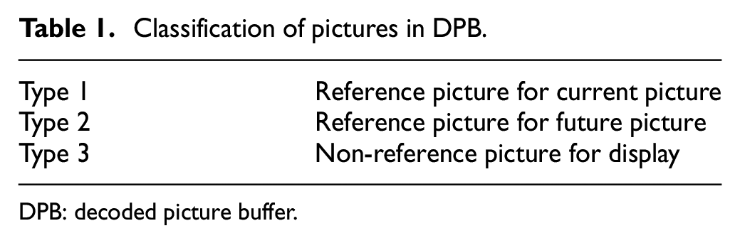
DPB: decoded picture buffer.
Type 1 is stored in the DPB as a reference picture to encode the current picture. Type 2 is not used as a reference picture to encode the current picture, but is stored in the DPB as a reference picture to be used in the future. Type 3 is not used as a reference picture but is stored in the DPB to display the video according to the picture order counter (POC). The HEVC encoder and decoder construct an RPL using pictures corresponding to Type 1. Up to two RPLs are used, and are divided into two RPLs (List 0 and List 1). List 0 is composed of pictures whose POC is before the picture to be coded, and List 1 is composed of pictures whose POC is later than the picture to be coded.
Figure 1 shows the process of constructing the RPL. When the current picture to be coded is a P-picture, only List 0 is configured. In the case of a B-picture, both List 0 and List 1 are configured to perform bi-directional prediction. When the process of constructing the RPL is started, List 0 is preferentially inserted negative short-term picture which has a temporally short distance of lower POC value based on the current picture to be coded. If the available negative short-term picture fails to fill all of the RPL, a positive short-term picture is inserted in List 0, which is temporally short distance and the POC value is higher than the picture to be coded. If the picture of the sum of negative short-term pictures and positive short-term pictures fails to fill all of the RPLs, a long-term picture that has a temporally long distance of the current picture to be coded is inserted to construct List 0. When the configuration of List 0 is completed, it is determined whether the picture to be encoded is a B-picture. If the picture is not a B-picture, the process of constructing the RPL is completed, and if it is B-picture, the List 1 process of constitution is started. List 1 is preferentially inserted with a positive short-term picture that has a temporally short distance of higher POC based on the current picture to be coded. If the available positive short-term picture fails to fill all of the RPL, a negative short-term picture is inserted in List 1, which is temporally short distance and the POC value is lower than the picture to be coded. If the picture of the sum of positive short-term pictures and negative short-term pictures fails to fill all of the RPLs, a long-term picture that has a temporally long distance of the current picture to be coded is inserted to construct List 1 and the RPL construction process is completed. As an example of the process of constructing RPL, Figure 2 shows an example of the prediction structure of random access encoding mode for the first 17 pictures. Table 2 shows examples of List 0 and List 1 according to each POC through the process of constructing RPL in the prediction structure of Figure 2. 30

RPL construction process.

Example of prediction structure of random access encoding mode for the first 17 pictures.
Constructed RPLs for the first 17 pictures of a sequence coded with the reference picture sets from Figure 2.
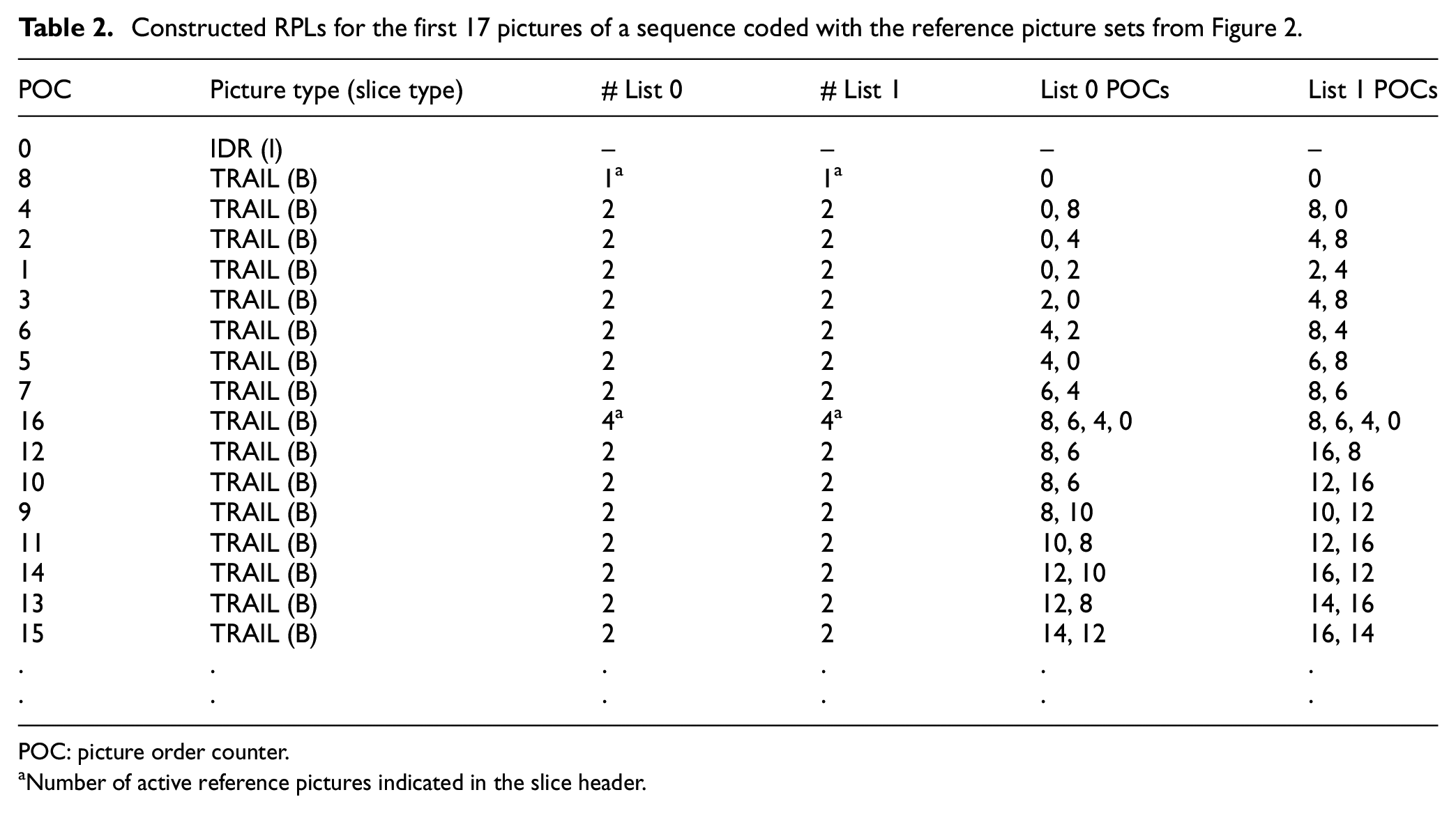
POC: picture order counter.
Number of active reference pictures indicated in the slice header.
Fast inter-coding using scene-change information of input video
The reference structure of the inter prediction in HEVC is performed within the GOP. For example, if the size of the RPL is two in the GOP structure composed of eight pictures, as shown in Figure 3, List 0 of POC 1 is composed of POC 0 and POC 2, and List 1 is composed of POC 2 and POC 4. An optimal prediction block is found through ME from these reference pictures and a prediction block is generated through MC. If scene change occurs in POC 4, POC 1 performs ME and MC for POC 0 or POC 2. Furthermore, POC 1 must perform ME and MC for POC 4. If the RPL is reconstructed by knowing in advance the point where the scene change occurs, the calculation complexity could be reduced since the ME and MC for the POC 4 are not performed.

Prediction structure in the random access encoding mode.
Scene-change detection
Videos have an inherent hierarchical structure and consist of frames, shots, and scenes, as shown in Figure 4. A shot is a series of pictures taken from the same camera that runs without interruption for a period of time, while a scene is a series of consecutive shots. 31 The most common scene change is the change of scene with cut of camera. One way of finding such cut points is to determine the boundaries between consecutive camera shots.

Inherent hierarchical structure of video sequence.
In this article, we detect the scene change before beginning the encoding process. Since the required preprocessing is performed before the encoding process, we adopt a well-known simple scene-change detection method. Pixel differences between two adjacent pictures are used as a comparison measure. The absolute frame difference (AFD), Dij, used for pixel-based scene-change detection for each input picture is calculated as follows

where p(n) denotes luminance value of each pixel in the nth picture within the range of 0–255, and i and j designate the position of each pixel in the picture. Using the Dij obtained from equation (1), the number of Dij values that are greater than a threshold DT is counted as follows

We empirically observe that most AFD values lie below a certain threshold, implying that they are unlikely to be scene-change pictures. According to Yi and Ling, 32 the appropriate DT value has been determined to be 35. If Count(Dij) is greater than a certain threshold T, we decide that a scene change has occurred in the current picture, as shown in the following equation

Threshold T is critical to the performance of the scene-change detection. Figure 5 shows the distribution of the number of Dij that is greater than 35 (which corresponds to Count(Dij)) for the 180 pictures with various video resolutions. For this experiment, we used the 1–15 sequence 33 of “The SJTU 4K video sequence dataset” provided by Zhao Tong University (SJTU) to construct three sets of test sequences containing scene changes. To obtain various scene-change effects, it is generated by concatenating the 1–15 sequences in an arbitrary order. In Figure 5, if there is no scene change in a picture, very small AFD is observed. Otherwise, a much larger AFD could be observed. This characteristic can be observed regardless of the video resolutions. In this experiment, we set the T value of equation (3) to be 1/2 (denoted as T1/2), 1/4 (denoted as T1/4), and 1/8 (denoted as T1/8) of the total number of pixels. From the results shown in Figure 5, we notice that when the T value is T1/2, false detection of a scene change has occurred. There are two false detections in Figure 5(a), two in Figure 5(b), and three in Figure 5(c). On the contrary, accurate scene-change detection could be achieved using T1/4 and T1/8 as the T value. Accordingly, we select the T value as T1/4 and T1/8. We observe similar results for various other test video sequences.

Experimental results on Count(Dij) to determine scene changes for various video resolutions: (a) 3840 × 2160 resolution, (b) 960 × 540 resolution, and (c) 120 × 68 resolution.
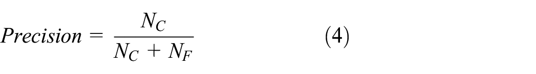
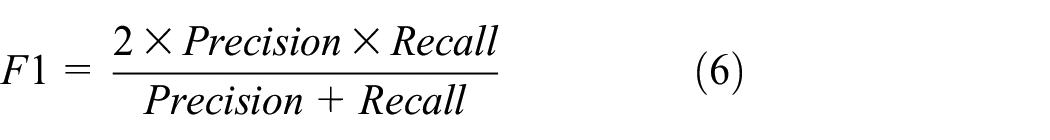
Table 3 shows the experimental results on the scene-change detection accuracy and the time required according to various video resolutions. For the performance evaluation of scene-change detection, we employed Precision, Recall, and F1, which are well-known criteria to measure scene-change detection accuracy, as shown in equations (4)–(6). Precision is the ratio of correct detections to the overall declared number of events. Similarly, the Recall parameter defines the ratio of true detections to the number of overall scene changes. F1 is a measure that combines the precision and the recall. In equation (4), NC indicates the number of correctly detected scene changes, and NF denotes the number of wrongly detected scene changes. The variable NM shown in equation (5) indicates the number of missed scene changes. If a scene change occurs but is not detected, NM is counted. On the other hand, NF is counted when no scene change occurs but is detected

Experimental results for various video resolutions in terms of scene-change detection accuracy and processing time.

N/A: not applicable.
According to the results shown in Table 3, all the T value cases show perfect Precision performance, while the T value case of T1/2 shows inferior Recall and F1 performance compared to other T value cases. For the T value cases of T1/4 and T1/8, all the same perfect Precision, Recall, and F1 performances are observed regardless of the video resolutions, since there is no substantial difference in scene characteristics between high- and low-resolution video. Therefore, it is more advantageous to use lower-resolution video than high-resolution video to detect scene changes in terms of required computational complexity and detection accuracy. Actually, as shown in Table 3, around 63 s is required to detect scene changes for the original 4K-UHD (3840 × 2160) video, while it takes 31.1 s for down-scaling the 4K-UHD to 120 × 68 resolution and 0.05 s for scene-change detection of the down-scaled video, resulting in a total of 31.15 s. Therefore, we can reduce the total processing time by about 50%, while obtaining the best scene-change detection accuracy using the down-scaled video and proper T values.
Proposed algorithm
Figure 6 shows the preprocessing workflow for scene-change detection, which is applied before HEVC encoding. For the input video, down-scaling is performed to reduce the amount of computation required for scene-change detection. The scene-change points of input video are identified by applying the pixel-based scene-change detection algorithm described in section “Scene-change detection” to the down-scaled video. We use the obtained scene-change points to distinguish POC groups in the GOP. For every new scene-change point, the POC group value is incremented by 1.

Preprocessing workflow for scene-change detection.
The proposed algorithm is described using an example illustrated in Figure 7. Figure 7 shows an example of the prediction structure of the HEVC encoding based on the POC group values obtained through the preprocessing when the scene change occurs in POC 4. In this case, the POC group value is increased from 0 to 1, and the POC group value will be increased from 1 to 2 if an additional scene change occurs thereafter. The POC group values are used to reconstruct the RPL.

Example of prediction structure based on the POC group values.
Figure 8 shows the proposed flowchart for the RPL reconstruction using POC group values obtained through the preprocessing. Note that the proposed algorithm is executed only when the current picture’s temporal level is greater than 1. The POC group value of the current picture (Curr_POCGroup) is compared with the POC group value of the pictures in the RPL (Ref_List0_POCGroup and Ref_List1_POCGroup). If the POC group value of the current picture is the same as that of the pictures in the RPL, the current picture is stored in the RPL. Otherwise, it is not stored.

Proposed flowchart for the RPL reconstruction using POC group values.
Table 4 shows the referenced POCs in List 0 and List 1 for the case of Figure 7 based on the proposed algorithm to reconstruct the RPL using the POC group values. According to the results, we can observe that there have been changes in referenced POCs in RPL by referring to POC group values. Using the POC group value, RPL is only composed of reference pictures that have an equal POC group value with the current picture. Accordingly, we can achieve significantly reduced encoding time, since we can avoid unnecessary computations required to predict the current picture from other dissimilar reference pictures.
Referenced POCs in List 0 and List 1 for the case of Figure 7, based on the proposed algorithm.

POC: picture order counter; N/A: not applicable.
Experimental environments and data set
The experimental computing environments employed for the performance comparison are shown in Table 5. The proposed algorithm is implemented on top of HM 16.12 reference software 34 to evaluate the performance in terms of computational complexity and encoding time. For the experiment, the encoding is performed in the random access mode and we adopt DownConvert in SHM-9.0 35 for down-scaling in the preprocessing. The experiments are carried out by modifying the conventional setting values related to FEN (fast encoder decision) and FDM (fast decision for merge) RD cost, which are fast coding tools of HEVC encoder.
Experimental computing environments.

RAM: random access memory; OS: operating system.
Table 6 is a list of source videos to be randomly cut and concatenated to create test video sequences containing various types of scene changes. The source videos are provided from “The SJTU 4K video sequence dataset,” 33 “The Ultra Video Group database,” 36 and “MCML 4K UHD video quality database.” 37 Table 7 shows the created test sequences used as input video in the experiments. They have two types of resolutions with various frame rates and contain seven or eight scene-change points. To create the 4K-UHD resolution test sequences with frame rate of 120, the seven source videos of the ultra video group are arbitrarily combined. To obtain the 4K-UHD resolution test sequences with frame rate of 60, frame-rate down conversion is applied to the 4K-UHD resolution test sequences with frame rate of 120. The test sequences with frame rate of 30 are generated by arbitrarily combining the source videos from SJTU and MCML Group. To create the test sequences with full-HD (FHD) resolution in Table 7, the 4K-UHD test sequences are down-scaled to FHD and are processed following the same procedure as above.
List of source videos used to create test sequences.

Created test sequences.

UHD: ultrahigh definition; FHD: full HD.
Experimental results
Table 8 shows the elapsed time for the preprocessing including down-scaling and scene-change detection. The scene-change detection time is observed to be only 0.05 s, on average, and the elapsed average time for down-scaling to 120 × 68 resolution is measured to be 16.54 s for 4K-UHD and 7.53 s for FHD. From the preprocessing, we could obtain significant information in advance, which is essential to reduce the HEVC encoding time. The elapsed overhead time for preprocessing can be compensated by significantly reducing the HEVC encoding time.
Elapsed time for down-scaling and scene-change detection required for preprocessing.

FHD: full-HD.
Table 9 shows the coding gain of the proposed algorithm over HM 16.12 in terms of compression efficiency and processing time for encoding. To verify the effectiveness of the proposed algorithm in terms of processing time, the processing time gain ΔT is used as a measure of complexity reduction

where tHM16.12 represents the normal HEVC encoding time and tproposed denotes the actual processing time for the HEVC encoding incorporating preprocessing in the proposed algorithm.
Coding gain of the proposed algorithm in terms of compression efficiency and processing time (using scene-change information only).
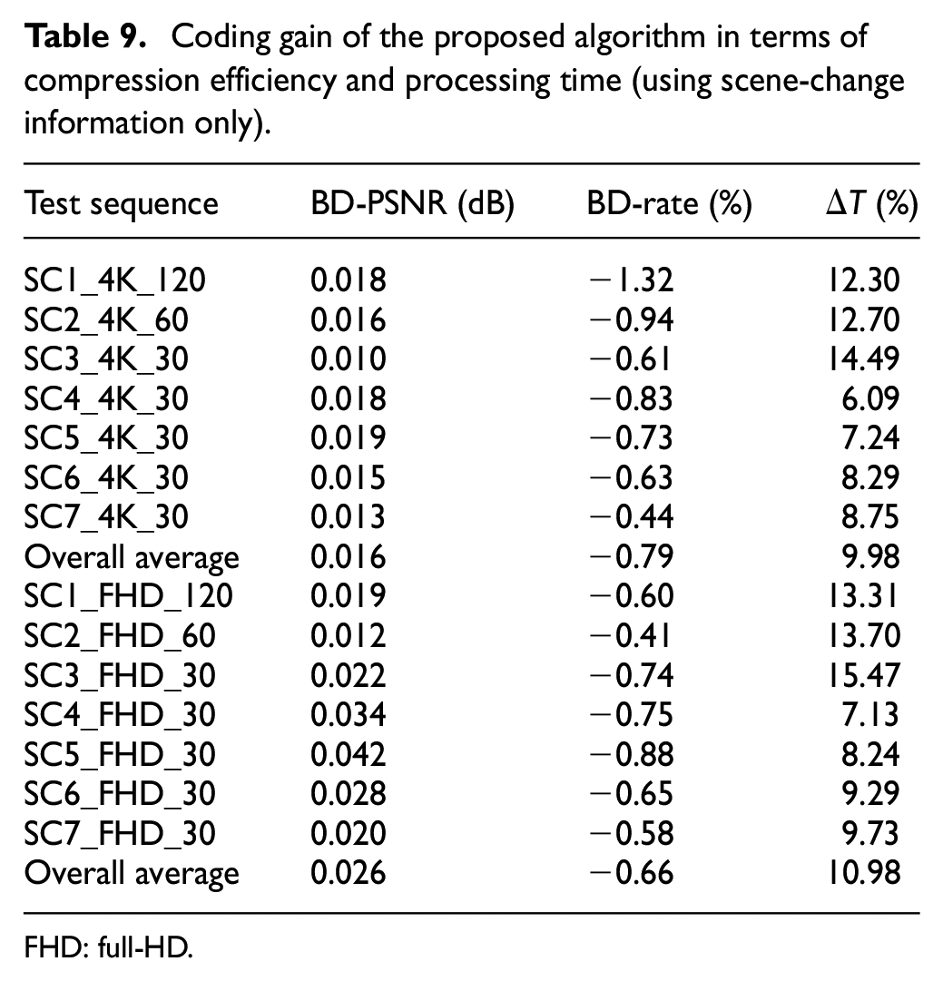
FHD: full-HD.
As for the compression efficiency comparison for 4K-UHD video, we could achieve Bjøntegaard Delta (BD)-PSNR improvement by 0.016 dB, on average, by the proposed algorithm, while achieving BD-rate reduction of 0.79% at the same time. On average, ΔT gain of 9.98% could be achieved by the proposed algorithm for 4K-UHD video. This means that the total processing time incorporating both the preprocessing and the HEVC encoding is significantly less than the total encoding time required by the normal HEVC encoding adopting HM 16.12. For the case of FHD video, the BD-PSNR is improved by 0.026 dB, on average, and the BD-rate is reduced by 0.66% with ΔT improvement of 10.98% on average.
The encoding performance by the proposed algorithm could be further improved by combining fast coding modes based on FEN and FDM parameters. The main idea of FEN is that the following CU calculation is skipped when the RD cost of the current CU, which selects SKIP mode as the best mode, is smaller than the average RD cost of previously encoded CUs. The FDM avoids computation of the RD cost of the merge mode for some merge candidates based on the early termination rule. Both fast coding modes commonly provide improved coding efficiency when a more similar reference picture to the current picture is used for prediction. In the proposed algorithm, the RPL is reconstructed with more similar reference pictures to the current picture by considering the identified scene-change points. Thus, the similarity between the current block and the neighboring blocks in the reference picture that are used to determine the merge and SKIP mode is increased. This increases the number of merge and SKIP modes during the fast coding and results in improved coding efficiency. Table 10 shows the improved encoding performance when the fast coding modes are combined with the proposed algorithm. As shown in Table 10, the BD-PSNR could be improved by an additional 0.014 dB relative to values without fast mode for the 4K-UHD video. The BD-rate could be reduced by an additional 0.61% with additional processing time saving of 7.69% on average. For the case of FHD videos, the BD-PSNR could be additionally improved by 0.011 dB relative to performance without fast mode, and the BD-rate could be additionally reduced by 0.27% with additional processing time saving of 7.75% on average.
Comparison of encoding performance between “with fast mode” and “without fast mode” (using scene-change information only).

FHD: full-HD.
Figure 9 shows the graphical comparison of encoding performance between “with fast mode” and “without fast mode” for various 4K-UHD input videos based on the results of Table 10. According to Figure 9, by combining the proposed algorithm with the fast coding mode of HEVC encoding, we could obtain considerable improvement in the encoding performance relative to the “without fast mode” case. In general, as the correlation among the reference pictures becomes higher, better encoding performance can be accomplished under the fast coding mode. By applying the proposed preprocessing, pictures with similar scene characteristic in the RPL become associated with the same POC group, thereby resulting in improved encoding performance. Therefore, it is expected that the proposed preprocessing can be more effective when it is combined with various conventional fast inter prediction algorithms.
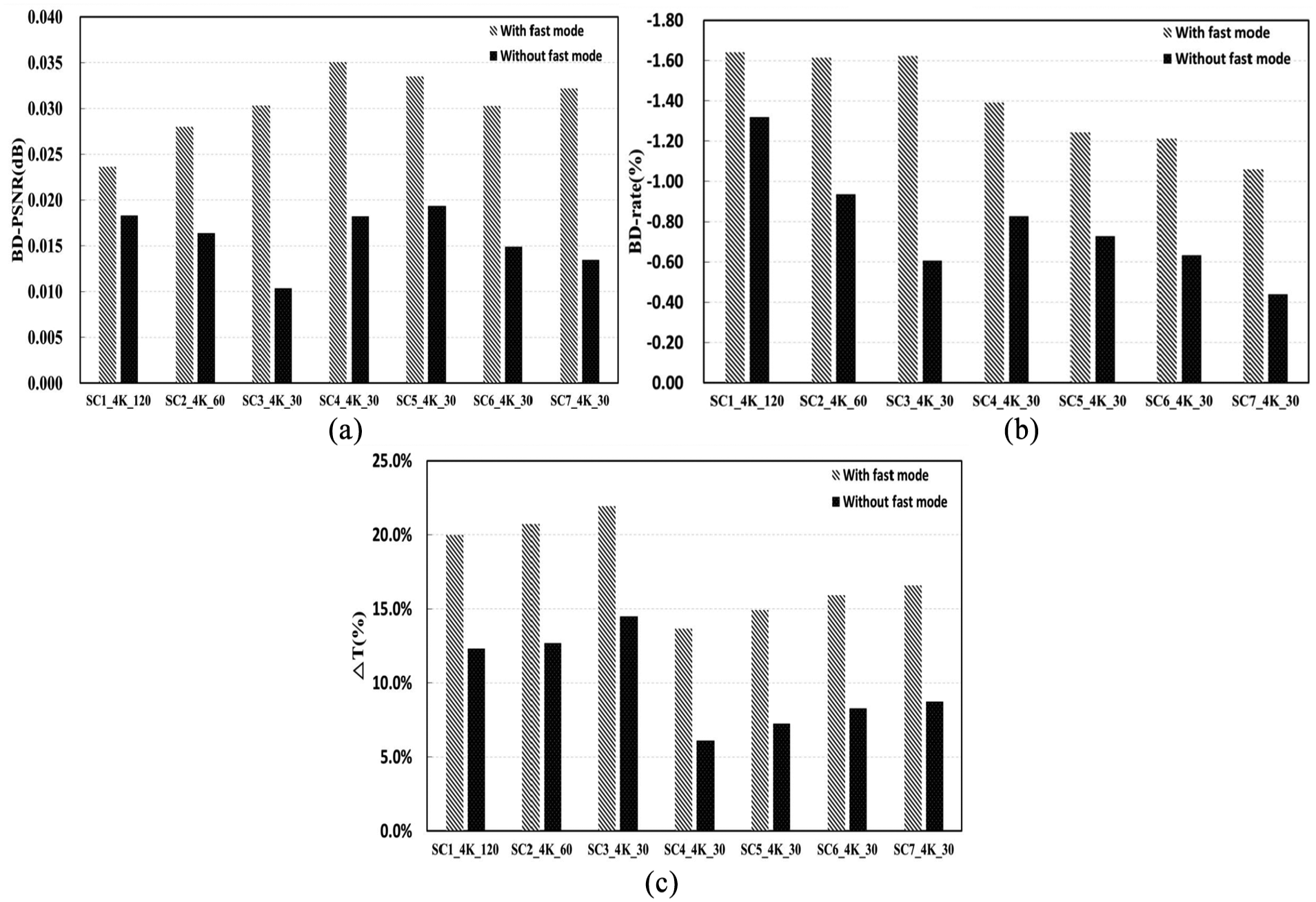
Graphical comparison of encoding performance between “with fast mode” and “without fast mode” for various 4K-UHD input videos: (a) improved BD-PSNR, (b) reduced BD-rate, and (c) processing time gain (using scene-change information only).
Fast inter-coding using scene-change information and GLCM of input video
The RPL for inter prediction inserts short-term pictures having the shortest inter-frame distance from previously coded pictures, as shown in Figure 1. For example, if the size of the RPL is 2 in the GOP structure composed of eight pictures, as shown in Figure 3, the List 0 of POC 1 is generally composed by POC 0 and POC 2, and the List 1 is generally composed by POC 2 and POC 4. However, inserting a list of reference pictures that is most similar to previously coded pictures instead of simply considering the shortest inter-frame distance can reduce the calculation complexity of ME and MC processing, since we can reconstruct the RPL by which we can obtain the motion information of the current picture to be the most similar to that of the reference picture. For that propose, we use the statistical characteristic indicators for the pictures of input video by exploiting GLCM and sort the RPL based on that information.
GLCM
In the image processing, the texture information of images is mainly used for analysis of satellite photographs, classification of videos, and recognition of medical images such as microscopic photograph analysis of living tissues. Texture is a characteristic that is important in image analysis. The texture of the image represents the spatial distribution pattern of the luminance change in the image. One pixel in a picture cannot represent the nature of a texture, and the texture is expressed by its relationship with neighboring pixels. This texture analysis method is divided into a structural method of dealing with the regular space arrangement of the picture prototype and a statistical method of analyzing the correlation between each pixel in a picture. Since the structural method uses only the luminance value of the object without using information about the position or shape of the object, there is a disadvantage in that the analysis can be performed only if the circular structure in the picture has a large and constant rule. The statistical method uses a method of recognizing and separating the spatial characteristics included in the original picture. To do this, a basic statistic is calculated between neighboring pixels included in a mask window which is constant around a target pixel. This makes it possible to extract new information and results that are not present in the original picture and to determine the spatial characteristics. One of the typical techniques for analyzing the texture characteristics of picture is the GLCM. GLCM is a two-dimensional gray-level histogram that transforms a pair of pixels into a fixed spatial relationship and analyzes the texture based on the secondary statistic. GLCM proposed a basic concept for pixel-based statistical texture image analysis. 38 The GLCM uses the luminance of each pixel in the gray-level picture to represent the frequency of occurrence of the relationship between the contrasts of neighboring pixels to a matrix. Franklin et al., 39 Kiema, 40 and Herold et al. 41 performed studies on the applications of satellite images such as agricultural and urban environment analysis studies on texture images generated based on GLCM.
The matrix P of the GLCM is represented by a four-dimensional matrix of distance (d), direction (θ), and gray-level pair i and j. P[d, θ, i, j] is the number of all pixel pairs whose gray levels are i and j, respectively, for pixel pairs that are separated by distance d in the θ direction. The GLCM, the unnormalized frequency of the function P(d, θ, i, j) of the θ quantized in the interval of 45 from the distance d in the M × N gray-level picture, is given by equations (8)–(11)


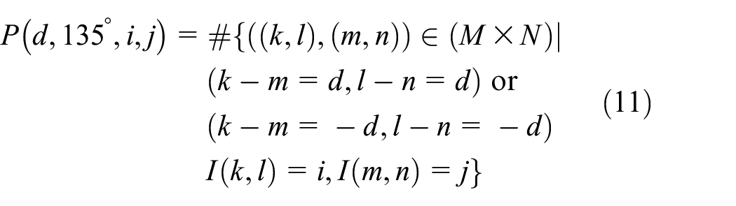
In the equations, I(k, l) denotes the gray level value of the pixel corresponding to the (k, l) coordinate of the M × N gray-level picture, and # denotes the number of set elements. The GLCM first determines the distance d and the direction θ of the pixel pair to generate P[i, j]. The distance d and the direction θ of the pixel pair are expressed by the displacement vector D = (dx, dy). dx is the amount of change on the x-axis coordinate between two pixels, and dy is the amount of change on the y-axis coordinate between the two pixels. The function P(d, 0°, i, j) with distance d and 0° in equation (8) means GLCM P[i, j] with displacement vector D = (d, 0). The distance set in the generation of the GLCM can be calculated by applying various values from 1 to 10. However, generally, when a large distance value is applied to a picture having a complex texture, a GLCM that cannot obtain detailed texture information is generated. 42 Therefore, the best results can be obtained when the distance is 1 or 2. 43
Figure 10 shows the direction and displacement vectors of the GLCM. Neighboring pixels considered in the center of the pixel have eight directions (0°, 45°, 90°, 135°, 180°, 225°, 270°, and 315°). However, according to the definition of GLCM, the simultaneous pixel pair is obtained when θ = 0° is the same as when θ = 180°. Therefore, in Figure 10, directions 1 and 5 are 0° (horizontal), 3 and 7 are 90° (vertical), 2 and 6 are 135°, and 4 and 8 are 45°. Only four directions are used in the GLCM. Since the row and column values of the GLCM are determined by the gray level, the higher the value of gray levels, the higher the computational complexity and the more accurate texture characteristics can be analyzed.

The direction and displacement vector of GLCM.
To represent the GLCM numerically, three indices were developed in the work by Haralick et al., 38 after which new indicators were developed and seven indicators were used. 44 Among these indicators, the formula of Contrast (CON), Dissimilarity (DIS), Homogeneity (HOM), Angular Second Moment (ASM), Energy (ENG), Entropy (ENT), and Correlation (COR), which are used for statistical characteristic indicators for texture analysis, has been generally employed. Homogeneity and Dissimilarity are applied differently according to the contrast of pixels. Homogeneity is a concept that represents the uniformity of each pixel. The Homogeneity has the largest value when the values of the elements in the GLCM are close to the diagonal. Contrast and Dissimilarity are used to distinguish inter-pixel differences in luminance. Higher weights are applied to pixels that are relatively far from the diagonal, and higher values are obtained when the number of pixels having a large difference in luminance is large. ASM and Energy are the indicators for measuring the uniformity of luminance. Unless there is a change in luminance between the pixels, the value of element of GLCM becomes a similar value so that it has a large value. Entropy is the indicator that can measure the randomness of the luminance distribution. Since the luminance of a pixel varies greatly, the value of the element of the GLCM becomes large when it is distributed in various places. Correlation between pixels means that there is a predictable and linear relationship between the two neighboring pixels within the window, expressed by the regression equation. A high correlation texture means high predictability of pixel relationships. 45 For more details on the seven indicators, see the work by Liu et al. 44
Proposed algorithm
Figure 11 shows the preprocessing workflow for the RPL sorting, which includes image texture calculation using GLCM. For the image texture calculation, we employed ASM, Contrast, Entropy, and Correlation indicators, which are essential elements to measure similarity between the current and reference pictures. These statistical features are calculated in four directions (0°, 45°, 90°, and 135°) for each picture, resulting in 16 statistical characteristic values in total. To find out the most similar picture in the reconstructed RPL using POC group values, the following similarity measure based on Euclidean distance is used


Preprocessing workflow for the RPL sorting.
where pi denotes the ith value of the 16 indicator values of the current picture p, qn,i denotes the ith value of the 16 indicator values of POC n. As illustrated in Figure 3, if the current picture is POC 3, the corresponding n is 0, 2, 4, and 8. Smaller similarity values indicate greater similarity of the picture to the current picture. Using equation (12), we reconstruct the RPL according to the similarity measures.
Figure 12 shows the proposed flowchart for the RPL reconstruction using not only POC group values but also the similarity measure obtained through the preprocessing. First, using the POC group value, we compose POC group List 0 for the current picture. Thereafter, if POC group List 0 has more than one reference picture, we calculate distqn values for the current picture and sort them in ascending order. Otherwise, we skip calculating distqn values for the current picture. After composing List 0, we construct List 1 by checking whether the current picture is B-picture or not. If the current picture is B-picture, we follow the same process as List 0. Otherwise, the RPL reconstruction for the current picture is terminated.

Flowchart for the RPL reconstruction using not only the POC group values but also the similarity measure obtained through the preprocessing.
For the case of Figure 7, where the GOP is divided into subgroups using the POC group value that is obtained by preprocessing, Table 11 compares the POCs in List 0 and List 1 between RPL reconstructions using only the POC group values and RPL reconstruction using the similarity measure in addition to the POC group values. According to the results, we can observe that there have been changes in POC values in RPL for several current pictures having POC of 3, 6, and 7. Using the changed POC value, we can achieve more improved compression efficiency since the new reference picture corresponding to the changed POC value shows higher similarity with the current picture, which is essential to advanced inter-frame prediction.
Comparison of POCs in RPL depending on using scene-change detection and GLCM for Figure 7 case.

POC: picture order counter; RPL: reference picture list; GLCM: gray-level co-occurrence matrix; N/A: not applicable.
Experimental results
The experimental environment employed for the performance comparison is the same as described in section “Experimental environments and data set.” The proposed algorithm is implemented on top of HM 16.12 reference software 34 to evaluate the performance of RPL reconstruction, compression efficiency, and encoding time. Table 12 shows the elapsed time for the preprocessing including down-scaling, scene-change detection, and GLCM texture calculation. The GLCM texture calculation time for the GLCM gray level of 64 is measured to be 0.36 s on average, which is a trivial overhead, and the scene-change detection time is observed to be only 0.05 s on average. The elapsed average time for down-scaling to 120 × 68 resolution is 16.54 s for 4K-UHD and 7.53 s for FHD. From the preprocessing including GLCM texture calculation, we could obtain significant information in advance, which is essential to reduce the HEVC encoding time.
Elapsed time for down-scaling, scene-change detection, and GLCM texture calculation for preprocessing.

GLCM: gray level co-occurrence matrix; FHD: full-HD.
Table 13 shows the coding gain of the proposed algorithm over HM 16.12 in terms of compression efficiency and processing time for encoding. To verify the effectiveness of the proposed algorithm in terms of processing time, the processing time gain ΔT in equation (7) is used as a measure of complexity reduction. Regarding the compression efficiency comparison for 4K-UHD video, it is found that the BD-PSNR could be improved by 0.037 dB, on average, by the proposed algorithm. At the same time, we could reduce the BD-rate by 1.53% on average. As for the ΔT gain, we could achieve 8.43% reduction in processing time, on average, for 4K-UHD video. In the case of FHD video, the BD-PSNR is improved by 0.049 dB, on average, the BD-rate is reduced by 1.28%, and the processing time is improved by about 9.49% on average. The results show that the compression efficiency can be improved by reconstructing RPLs using pictures with high similarity through image texture calculation using GLCM. When comparing the processing time gain with that of Table 9, GLCM-based fast inter-coding does not exhibit superior performance improvement in terms of encoding complexity reduction. This is due to the fact that image texture calculation using GLCM requires an additional processing time. However, this defect could be overcome by employing an optimized GLCM calculation method. Furthermore, if we could obtain even the scene-change information by using GLCM, this would result in a significantly improved time complexity.
Coding gain of the proposed algorithm in terms of compression efficiency and processing time (using both scene-change information and GLCM).

FHD: full-HD.
Figure 13 compares PSNR performance between HM 16.12 and the proposed algorithm described in section “Proposed algorithm.”Figure 13(a) shows experimental results for the SC6_4K_30 test sequence. According to the results, the proposed algorithm shows superior PSNR performance to the HM 16.12 over all the bit rate ranges. In particular, note that, as the bit rate increases, the PSNR gap between the proposed algorithm and the HM 16.12 is proportionally increased. For a given higher bit rate, the finer quantization scale is used to generate more bits and results in better visual quality in general. Therefore, in the proposed approach, the reconstructed RPLs during the encoding process have enhanced visual quality and they are used as reference pictures for the prediction. This results in improved prediction and PSNR performance since the reference pictures in the RPL used for prediction have better visual quality and contain much more similar visual content to the current picture than the conventional HM 16.12. Figure 13(b) shows experimental results for the SC5_FHD_30 test sequence. Conducting the same analyses in Figure 13(b), we observe similar tendencies to the results shown in Figure 13(a).

Comparison of PSNR performance between HM 16.12 and the proposed algorithm: (a) SC6_4K_30 (3840 × 2160) and (b) SC5_FHD_30 (1920 × 1080).
The encoding performance by the proposed algorithm could be further improved by combining fast coding modes based on FEN and FDM parameters. Table 14 shows the improved encoding performance when the fast coding modes are combined with the proposed algorithm. As shown in Table 14, the BD-PSNR could be additionally improved by 0.019 dB relative to the performance without fast mode for the 4K-UHD video, and the BD-rate could be additionally reduced by 0.76% with additional processing time saving of 8.02% on average. For the case of FHD videos, the BD-PSNR could be additionally improved by 0.016 dB relative to the performance without fast mode. In addition, the BD-rate could be reduced by 0.38% with additional processing time saving of 7.91% on average. When comparing the results of Table 14 with those of Table 10, we can notice that the proposed algorithm using both the scene-change points and image texture information shows better compression efficiency performance than the algorithm using only scene-change points. This is due to the fact that the RPL could be reconstructed with much more similar reference pictures to the current picture by considering both the scene-change points and image texture information, thereby resulting in additionally improved encoding performance relative to the case of Table 10.
Comparison of encoding performance between “with fast mode” and “without fast mode.” (using both scene-change information and GLCM).
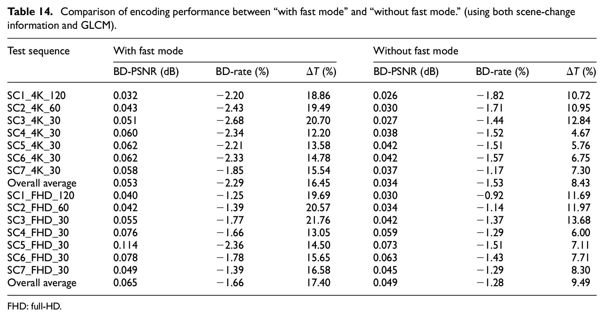
FHD: full-HD.
Figure 14 shows the graphical comparison of the encoding performance between “with fast mode” and “without fast mode” for various 4K-UHD input videos based on the results of Table 14. According to Figure 14, by combining the proposed algorithm with the fast coding mode of HEVC encoding, we could obtain significant additional improvement in the encoding performance than the “without fast mode” case.
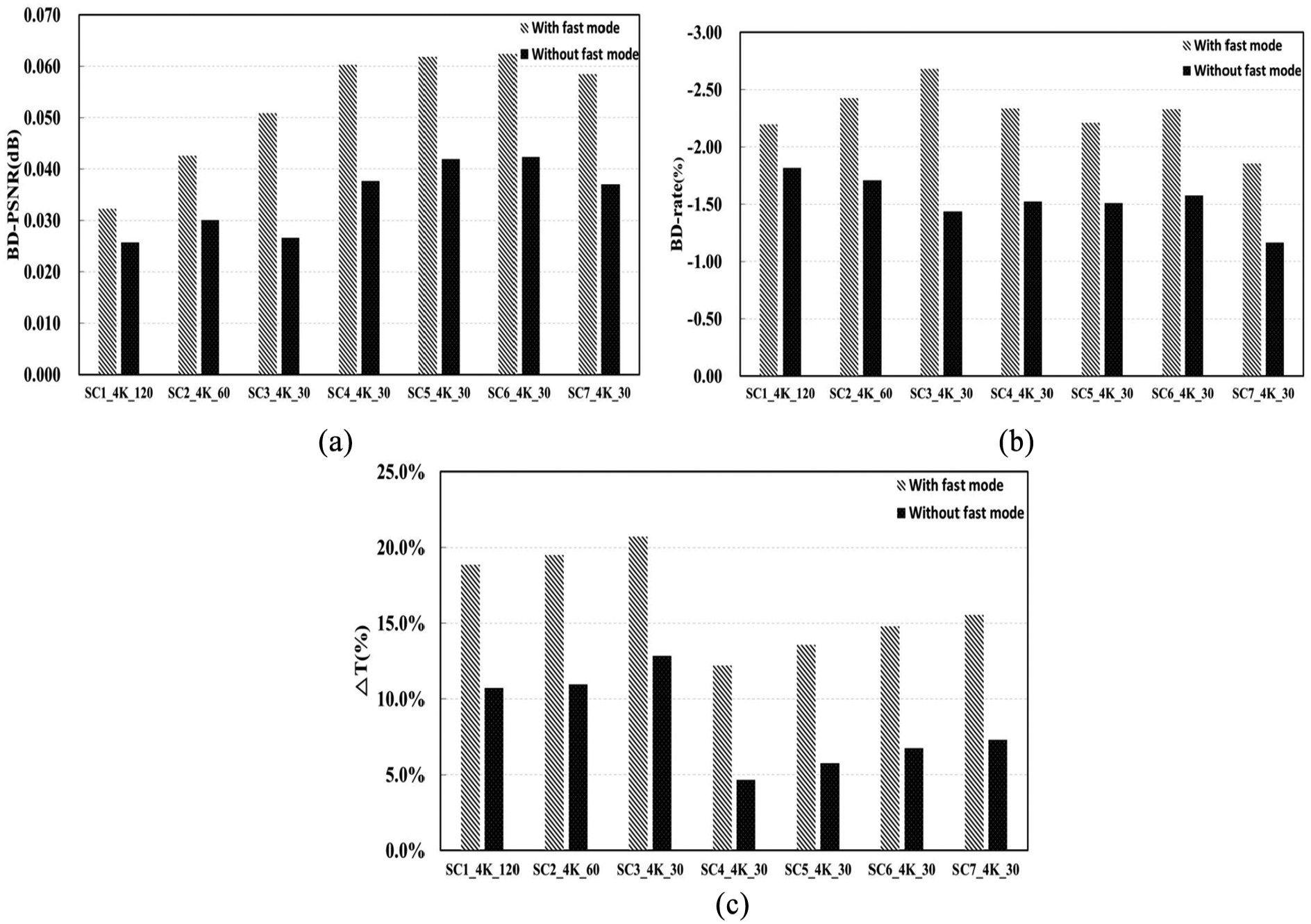
Graphical comparison of encoding performance between “with fast mode” and “without fast mode” for various 4K-UHD input videos: (a) improved BD-PSNR, (b) reduced BD-rate, and (c) processing time gain (using both scene-change information and GLCM).
Conclusion
In this article, we proposed a novel method of reconstructing the RPL for the fast inter-coding of HEVC. For this purpose, we employ advanced detection of scene-change points and exploit image texture information obtained from the input video because the fast coding–based conventional algorithms that employ the general RPL construction approach have difficulty in selecting a reference picture having high temporal redundancy (or high similarity to the current picture) for prediction. First, using the detection results of scene-change points, the RPL is reconstructed by selecting reference pictures with high temporal redundancy for prediction in the same scene. Accordingly, it is possible to achieve significantly reduced encoding time, since we can avoid unnecessary computations required to predict the current picture from the pictures with lower temporal redundancy in a different scene. Second, the image texture information is additionally applied to reconstruct the RPL by selecting an optimal reference picture that is the most similar to the current picture among the reference pictures. The reconstructed RPL improves the compression efficiency because the reference picture that is the most similar to the current picture is preferentially used for inter-frame prediction. Moreover, since the proposed algorithm selects the optimal reference picture based on similarity to the current picture, the analytic conditions for fast coding mode of HEVC occur frequently. This results in additionally improved encoding performance than the conventional fast coding–based algorithms that employ the general RPL construction approach. It is proven through extensive simulations that by combining the proposed algorithm developed for inter prediction with the conventional fast coding modes of the HEVC, the encoding time and coding efficiency could be significantly further improved. As a further work to additionally enhance the encoding speed, we are going to combine the proposed method with various analytic conditions such as CBF, ratio of SKIP mode, RD cost, and distribution of transform coefficients. The proposed algorithm incorporated with the HEVC can be practically applied to encode video sequences containing frequent scene cuts and high scene variation, such as entertainment videos, action movies, sports videos, and music videos.
Footnotes
Handling Editor: Bryan(Byung-gyu) Kim
Declaration of conflicting interests
The author(s) declared no potential conflicts of interest with respect to the research, authorship, and/or publication of this article.
Funding
The author(s) disclosed receipt of the following financial support for the research, authorship, and/or publication of this article: This research was supported by the Basic Science Research Program through the National Research Foundation of Korea (NRF) funded by the Ministry of Education (NRF-2018R1D1A1B07047065).