Sage Journals: Discover world-class research

Abstract

To discover road anomalies, a large number of detection methods have been proposed. Most of them apply classification techniques by extracting time and frequency features from the acceleration data. Existing methods are time-consuming since these methods perform on the whole datasets. In addition, few of them pay attention to the similarity of the data itself when vehicle passes over the road anomalies. In this article, we propose QF-COTE, a real-time road anomaly detection system via mobile edge computing. Specifically, QF-COTE consists of two phases: (1) Quick filter. This phase is designed to roughly extract road anomaly segments by applying random forest filter and can be performed on the edge node. (2) Road anomaly detection. In this phase, we utilize collective of transformation-based ensembles to detect road anomalies and can be performed on the cloud node. We show that our method performs clearly beyond some existing methods in both detection performance and running time. To support this conclusion, experiments are conducted based on two real-world data sets and the results are statistically analyzed. We also conduct two experiments to explore the influence of velocity and sample rate. We expect to lay the first step to some new thoughts to the field of real-time road anomalies detection in subsequent work.

Keywords

Acceleration data road anomaly detection cloud computing edge computing

Introduction

Road anomalies can lead to serious traffic accidents. For example, between 2000 and 2011, there were 2 million traffic accidents in Canada, of which 33% were related to road conditions or bad weather.¹ In 2015, about 50,000 British drivers were involved in traffic accidents caused by road anomalies, and road pits caused a car accident every 11 min.² As a result, governments spend huge amounts of manpower and resources on road maintenance. The British government announced that they spent $1.2 billion on road maintenance in 2007.³ In 2014, for the city of Toronto, Canada spent a total of $6 million on road repairs.⁴ Therefore, detecting road anomalies in an efficient and simple way is helpful to reduce the expense and improve efficiency of road repairs.

Traditional vision-based or laser-based road anomaly detection techniques are time-consuming or labor intensive.⁵ With the development of mobile devices and sensor technologies, it is possible to detect roadway anomalies using crowdsourcing-based sensor data. An anomaly is any permanent obstacle generated by the continuous use, weather conditions, or traffic planning decisions in the road. As the vehicle passes through the anomaly, the acceleration data imply an inherent pattern due to the type of anomaly. Thus, the problem is converted into detecting possible anomalies from sensor data.

Earlier work of Mohan et al.,³ Eriksson et al.,⁶ and Mednis et al.⁷ utilized threshold-based techniques to detect road anomalies. For example, some researchers^3,6,7 detected bumps and potholes. Although these methods can detect whether there is an anomaly, they cannot distinguish the type of anomalies. Furthermore, the detection accuracy is quite low. Recently, a few studies first extracted different kinds of features^7–12 and then used classification models^9,11–13 such as support vector machine, k-means, or decision tree. These methods suffer a few limitations: (1) they rarely filter out the impact of normal roads on model training; (2) the data between two anomalies in the same category may be similar in time domain, but none of them take this into consideration; and (3) they often use a fixed window length, leading to the possibility to slice anomalies’ data.

However, these methods take less consideration about how they apply their techniques into an operational way to help the government detect and report the road anomalies. Most of these methods^6,7,9 stop after a fine detection performance in a single road-device mode. A single road-device mode means the server processes an acceleration data series detected by one device from one specific road for one time even there are multiple roads in their data sets. Also, their methods process data locally and less consideration is put on the consumption when information is transferred from the device to the server. For the operational detection target, there should be multiple vehicles carrying one or two devices in each vehicle, and the vehicle would be running in different roads. We call it a multiple road-device mode. Under this mode, the application should be prepared to transfer information to the server; thus, the time, energy, or network consumption should be taken into consideration. However, the existing methods only focus on detection accuracy without considering the time consumption, the energy consumption, and the network usage. Some of them^2,11 utilized the data preprocessing, while the others paid more attention to the performance rather than the efficiency.

Under the consideration about reducing the consumption without loss in detection performance, we introduce the edge computing method in our implementation. That is to transfer some steps into the edge application in the device to reduce the size of information submitted to the server, as Figures 1 and 2 show, the data filter step. In fact, the ratio between normal road and anomalies is about 95:5 to 97:3,^2,14 and the anomalies only take a small portion. As a result of operating all the data and delivering them to the server, their methods take more time and consume more energy or network resource. If the anomalies are detected first and only the anomalies are sent to cloud server, time consumption of anomaly detection will be reduced greatly and thus enabling a real-time road anomaly detection system.

Figure 1.

Procedure of simulation for methods with data preprocessing.

Figure 2.

Procedure of simulation for methods without data preprocessing.

Taking these issues into consideration, this article focuses on the following:

Building a more realistic and meaningful situation where once a series of acceleration data is detected and a set of dynamic length anomalies are located and sent to the server to be determined as different types of anomalies.

Achieving better anomaly detection performance compared to some methods proposed in other papers;

Enabling a real-time road anomaly detection model in respect of delay, energy consumption, and network consumption with the simulation of edge computing software.

Our model can detect three kinds of anomalies: pothole, speed bump, and metal bump. In fact, only the potholes should be reported to the government, but the detection and identification of these types are necessary for the following:

From the perspective of the driver, the road anomaly detection program only needs to send information on whether there is an anomaly without determining the type of road anomaly; however, from the perspective of road maintenance personnel, judging whether an anomaly is a road pothole or a normal road equipment (speed bump or metal bump) is helpful for their work.

From the perspective of edge computing and cloud, the program judges the type of road anomaly and informs other drivers the type of road abnormality in a certain section through the cloud which is helpful for the improvement of the driving experience. Drivers will take different actions in the face of different types of road anomalies, such as decrease their speed before the speed bump and choose to avoid pothole and metal bump.

Judging the types of road anomalies can comprehensively evaluate the road conditions of a section of roads. Usually, drivers can notice speed bumps and metal bumps in a timely manner, so these road anomalies have less impact on a section of road conditions. When the cloud pre-notifies the driver, it only needs to remind the driver to keep a lower speed on the road with more potholes to get a better driving experience.

We utilize some existing data set to validate the effectiveness and efficiency of our method in different situations. Thus, our work can be the basis for subsequent road inspections such as formulating a road anomaly map of the city with the help of edge computing.^15,16

The contributions of this work are twofolds:

A threshold-based detection algorithm to extract the candidate anomaly window and a coarse classifier to filter out normal types from exception types are proposed based on the theory. The former one locates the possible position that might exists anomalies, and the latter one reduces time consumption and improves performance.

We compare our method with some existing methods and the proposed method demonstrated the least energy, time, and network consumption compared to both cloud-only and edge-ward methods.

This article is organized as follows. Section “Related work” reviews some related works during the past few years. Section “Overview of the proposed design” gives the main ideas and implementation of our method. Section “Experiment evaluation” presents the experimental results for multi-class anomalies classification, the performance of edge computing simulation and also the influence of velocity and sample rate to our method. Finally, section “Conclusion” concludes our work and predicts possible research directions.

Related work

Early studies mainly focus on threshold-based detection techniques to identify the anomalies. For instance, Mohan et al.³ proposed a system using acceleration information of the smartphone at a sampling rate of 310 Hz. Eriksson et al.⁶ detected road damage using a threshold-based filter with acceleration and GPS data at a sampling rate of 380 and 1 Hz in the Boston area. The system proposed by Mednis et al.⁷ used four heuristic threshold methods to detect road damage: Z-THRESH, G-ZERO, Z-DIFF, and STDEV. However, threshold-based detection method can only detect whether the road is damaged, but cannot identify the type of roadway surface disruption.

In recent years, many researchers believe that the extracting features from both time domain and frequency domain information can more accurately help to solve the problem. For example, Perttunen et al.⁸ used the fast Fourier transform and the Mel-frequency cepstral coefficient to obtain the energy value of each frequency band of the acceleration information and extracted a 95-dimensional feature for detection. Seraj et al.⁹ utilized wavelet transform to decompose acceleration data to extract feature vectors. Carlos et al.¹⁰ showed that the identification feature based on the standard deviation score can obtain better detection effect. El-Wakeel et al.¹¹ used wavelet denoising method to improve the quality of low-cost MEMS sensing data and made a roadway surface disruption based on the characteristics of time domain and frequency domain information extraction of acceleration. González et al.¹² took a word bag model to extract features from the acceleration data. Some researchers¹⁷ used some features such as the final stop duration or the number of stops of the car to characterize the road condition. Some researchers^18,19 took the angle of the road into consideration to modify the acceleration data, while some researchers²⁰ proposed some equations to use the acceleration data to discover the dimension of the pothole. Alessandroni et al.²¹ researched the relationship between the road roughness and the vehicle speed using their own model. Seraj et al.²² used 288 features per window to calculate the Euclidean distance. Madli et al.²³ established a rough judgment between the height or depth of road anomalies and the type of road anomalies.

One drawback of these studies is that first they do not think highly of the quantity difference between the normal road and the anomaly. According to data collected by some studies,^2,14 the ratio between normal road and anomaly is about 95:5 to 97:3. As a result, sliding window techniques² generate a large amount of windows that represent normal road, and it makes the procedure of SVM slow and inaccurate. Some methods¹⁴ used embedded platform to filter those normal road data, but it is complicated in design and cannot be applied to all mobile devices. Some researchers²⁴ used Gaussian model to predict the depth of the potholes. Also, some people²⁵ employed undersampled oscillation system to estimate the road surface.

The third disadvantage is that from a practical point of view, using a fixed window size in sliding window technique or making each anomaly included in a fixed time window after some processing may encounter the following issues: the division method can slice the anomaly into two windows and then the information of the anomaly decreases in both window, or the length of window can be less than the length of the anomaly data and then the anomaly cannot be perfectly covered by one window.

The last drawback is none of them consider to deploy their methods in a operational way. Some of them utilized the data preprocessing, while the others paid more attention to the performance rather than the efficiency. As a result, most of their methods need to transmit all the data to the server under the multiple device-road mode, which will generate more time, energy, and network consumption without doubt. These consumption needs to be reduced for the economic purpose.

Overview of the proposed design

Design framework

Because we introduce the edge computing step into the implementation, it is necessary to explain the entire step beyond the model. Our design is divided into two steps, namely, collecting data and training model off-line and user testing anomalies through the program online. We will discuss these two steps separately.

For the former step, the current method used in our experiments is to collect both acceleration data and the video and label the type, start time, and duration by video. Here is an example of how to label the type of anomaly as Figure 3 shows. The vehicle drives along the road and we put the mobile phone in the rear of the vehicle for the convenience of fixing. We found four significant frames in the video and marked the data series that there is a pothole. We only detect three anomalies that are significantly different; thus, it is easy to distinguish the type of anomalies. The judgment of start time or duration will be a bit difficult but can still be handled by locating the rapid change in acceleration data. For the future work, we will consider to introduce image processing technique to solve the problem of labeling the training set. Image processing is suitable for labeling a small amount of anomalies and can reduce the knowledge requirement. To check the effect of anomalies labeling, people only need to check whether an apparent anomaly in the video is labeled without the need to judge the duration or start time. This step is invisible for the model as it builds the whole database for the model to compare and calculate with. The database will be stored in the server.

Figure 3.

Illusion of the procedure to label anomaly.

For the latter step, it consists of all the procedures in Figure 4. The only work that non-professional people do is to download the application and open it no matter they are driving or sitting in a vehicle. In our design, the application will detect and submit the acceleration data belong to the anomalies to the server spontaneously. The server already sets up the model by previous database as training set, thus it uses the submitted data as a test set, generate the identification results and return the exact type of the anomaly to the application. From this perspective, non-professional people need no professional knowledge and will acquire what type the anomaly is. For the future work, drivers will previously get the road information to help them make driving decisions such as slowing down.

Figure 4.

The framework of the proposed anomaly detection and identification model.

In these two steps, we separate the professional knowledge from users that they only need and realize a design that separately figure out whether there is an anomaly in devices and what the anomaly type is in the server. We will focus on the online model in the following explanation. Our proposed model produces the detection and judgment result of an existing piece of data by three phases: (1) threshold detection and sliding window processing, (2) a quick filter of the normal window and the abnormal window, and (3) comparison to determine types using collective of transformation-based ensembles(COTE).

Threshold detection and sliding window processing

Figure 5 shows an example of the procedure of threshold detection and sliding window algorithm. This procedure is based on two facts that are observed throughout the data set:

If the vehicle drives in a normal road, the data of z-axis acceleration float in a certain range with a Gaussian noise.

Once driving over an anomaly, the data of z-axis acceleration often first exceed a high threshold and then fall under a low threshold or it behave in an opposite way, that is, first falling under a low threshold and then passing a high threshold. After this large vibration, it may continue to fluctuate in value and eventually fall back to the normal position.

Figure 5.

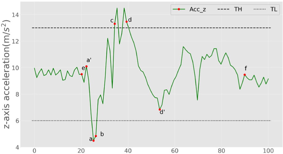
Illustration of threshold detection and sliding window.

With these two preliminaries, we suppose once the threshold point is detected, we can find the point at which the z-axis acceleration data starts to change and the point at which the z-axis acceleration data end to normal. Our candidate window will be located between these two points, which is probably an anomaly.

We take a pothole and its data as an example. It is supposed to start at point $e$ and end at point $f$ , as shown in Figure 5. First, point $a$ is found for the reason that the value of z-axis acceleration exceeds the high threshold $TH$ and its x-axis coordinate $x_{a}$ is marked. We set a parameter $Range$ for the reason that once a point over the high threshold is found, there should be at least one point that falls below the low threshold, according to our preliminaries. We suppose the last point that satisfies will cover the entire anomaly best, so we find it in a big enough range to cover most of anomalies in order not to miss any anomaly. Then, two points $a$ and $d$ are found. We compare the average value of the sliding window that begins from $a$ to $d$ , and when it starts to change, we will reach the final points of $a'$ and $d'$ .

A Quick filter of the normal window and the abnormal window

Windows in the candidate window set are not all windows generated from anomalies data. Only one-fourth of the total windows are abnormal windows. In order to exclude this part of the normal window, we observe some data and study the work of others and formulate a random forest model. The six features are the average value, the maximum and the minimum, the variance, the difference between the maximum or minimum, and the average value.

As Figure 6 shows, for the first window, we calculate the average value and the variance first, which are 10.2 and 7.6, respectively. After this, we find the maximum value and the minimum value of this window as 13.3 and 7.0, respectively. We separately calculate the difference between the maximum and the average value as 3.1 and the difference between the minimum and the average value as 3.2.

Figure 6.

The framework of training a random forest model and specifying anomalies.

For the second window, we calculate the value in the same way and the result as 9.8, 2.3, 11.1, 8.8, 2.3, and 1.0, respectively. For the remaining window, we do the same feature extraction work, and after collecting all features in all windows, we use the data in training set to train one random forest model with numbers of estimators as 10 and use this model to classify whether windows are anomaly windows. The first window is classified as anomaly window, while the second one is classified as normal one.

We reach the conclusion that the variance of z-axis acceleration when the vehicle drives through the anomaly will have a linear relationship with the depth or height of anomaly in the early research. Based on this conclusion, we mainly select some indicators that can reflect the change of acceleration as features to identify anomalies from normal road.

Another reason is that the fixed window, and not all abnormal windows, contains maximum or minimum in their methods. Often an anomaly window contains some points that belong to normal road, making the average closer to normal, and thus, the variance becomes smaller for anomaly window. As a result, the difference between maximum and average or the difference between minimum and average decreases. Our method does not have the effect of fixed window methods on features. The window would cover almost all information, thus the features become significant.

Using COTE to determine the type of anomalies

This step is mainly based on the idea of COTE algorithm according to Bagnall et al.²⁶ As Figure 7 shows, suppose our time series data have been normalized to zero mean and unit variance, we mark $p = m - l$ , where $m$ is the length of the data window and $l$ is the maximum lag. First, we calculate autocorrelation coefficient $r$ for $p$ times. This parameter describes the autocorrelation between variables $t_{i}$ and $t_{(u + k)}$ . After that, we formulate Toeplitz matrix $(π)_{p}$ of Advanced Custom Fields (ACF) terms and the first $p$ terms $R_{p}$ to figure out the associated set of parameters matrix $(δ)_{p}$ . This matrix will be a lower triangular matrix and the diagonal element will be our desired series $L$ . We apply the algorithm to the training window list and the testing window list, which contains some labeled anomalies.

Figure 7.

The framework of figuring out transformed data series $L$ .

Now that all the data are transformed, we select one testing window from the testing window list and calculate the Euclidean distance between the transformed testing data series and all the transformed training data series. After acquiring a list of distances between the selected testing window and the training window list, we apply k-nearest neighbor (KNN) algorithm to specify the type of this testing window. We apply this KNN comparison method to all the testing window list and acquire all the types of them.

Experiment evaluation

In this section, we will present the results of a series of experiments conducted to evaluate the performance of the proposed anomaly detection model. First, we describe the settings of experiments including data sets, compared methods, and evaluation metrics. Then, we will report and discuss the experiment results.

Experimental settings

Data sets

We utilize two data sets to validate the performance of our model and other existing methods.

Data set 1. This data set is based on the anomalies data that the paper² provides. In order to expand the scale of the problem to meet more realistic scenarios, we use all the anomalies data and normal road data and then randomly generate a road that contains every anomaly included in the data set. To simulate the real road in the real world, we insert anomalies into normal road in a realistic proportion according to the ratio of anomalies to normal road in existing data sets.^12,27,28 The ratio of the length of the anomalies to the normal road is set to 1:50.

Data set 2. This data set is inspired by the study by Fox et al.²⁹ to simulate and collect data from Carsim^®. We use the Carsim program to simulate vehicles driving over potholes, metal bumps, and speed bumps. With this tool, we simulated vehicles driving over 4000 potholes, 2000 metal bumps, and 2000 speed bumps. A large amount of accelerometer data is collected.

Data set 3. This data set is also generated by Carsim^®. We simulated vehicles driving over 100 potholes, 100 metal bumps, and 100 speed bumps with different velocity ranging from 10 to 100 km/h increasing at a 5 km/h step. The total size of the data set is 1900 potholes, 1900 metal bumps and 1900 speed bumps. We fix the sample rate at 120 Hz.

Data set 4. This data set is also generated by Carsim^®. We simulated vehicles driving over 100 potholes, 100 metal bumps, and 100 speed bumps with different sample rate ranging from 10 to 200 Hz increasing at a 10 Hz step. The total size of the data set is 1900 potholes, 1900 metal bumps, and 1900 speed bumps. We fix the velocity at 60 km/h.

The size of the four data sets is shown in Table 1.

Table 1.

Data sets and the size of anomalies.

Data set	Amount of pothole	Amount of speed bump	Amount of metal bump
Data set 1	236	138	135
Data set 2	4000	2400	2400
Data set 3	1900 (100 in each velocity)	1900 (100 in each velocity)	1900 (100 in each velocity)
Data set 4	1900 (100 in each sample rate)	1900 (100 in each sample rate)	1900 (100 in each sample rate)

Comparative methods

We compare the proposed recommendation model with the following four methods, all of which are popular work from the last 3 years.

SVM-WW. This method² was originally proposed to identify different anomalies such as potholes, metal bumps, and speed bumps based on z-axis data acceleration. Features are mainly some statistical indicators such as mean and standard deviation. They also proposed confidence score as feature to evaluate whether the statistical features are trustworthy.

CPD-SFS. This method¹⁹ was originally proposed to detect different lanes and to identify anomalies in different lanes. They managed to select most effective features by greedy forward selection algorithm and create some features that are more complicated such as the average of the absolute value of the product of z-axis acceleration and the velocity.

SVM-MDDP. This method¹¹ was originally proposed to identify various anomalies via sensor data based on multi-domain of processing. They first de-noised the data and then not only extracted statistical features like other literature, but also used time and frequency domain data and eventually achieved a feature scale of more than 70 dimensions.

MLM-WB. This method¹² was originally proposed to represent the time series data with some simplified representations called word bag. Basing on these representations, machine learning methods reached a higher accuracy.

We compare these methods with our proposed method, Quick filter with collective of transformation-based ensembles (QF-COTE). The results will be shown in the following section.

Evaluation metric

There are four main indicators for our evaluation: F1-score, average latency, average network usage, and energy consumption. For F1-score, it is calculated by the following equation

F 1 = \frac{2 TP}{2 TP + FP + FN}

(1)

In order to explain the problem more clearly, and to make our model closer to practical applications, we identify a true positive (TP) as the overlapping between the prediction and the real data,² as Figure 8 shows. The ground truth indicates the anomaly in the real world, and the predicted lines 1 and 2 are generated by some methods. The predicted line 1 and the ground truth overlap in time series 10–15, so we suppose the prediction is correct and it is a TP. The predicted line 2 and the ground truth do not overlap in any position, but there is a prediction, so it is a false positive (FP). In the real prediction situation, we want to know whether there is a anomaly on the road. We also want to know the specific location of the anomaly. However, predicting the true length of the anomaly is often unnecessary: the road maintenance department does not care about this type of information. As a result, this definition of TP is more reasonable. FP and false negative (FN) have similar definitions.

Figure 8.

Illustration of overlapping between prediction and ground truth to be a True Positive.

From the perspective of average latency, average network usage, and energy consumption, we utilize their software³⁰ to simulate the fog computing and we follow the metrics in this article. These metrics reflect the performance of different methods when they are deployed in fog computing situation.

Identification performance for all methods

For a comprehensive comparison, we adjust the validation part from 10% of the data set to 50% of the data set, to show the change of model performance under different scale of verification sets. As a result, the training part will grow from 50% to 90% by a step of 10%.

The results of data set 1 are illustrated in Figure 9. This data set includes a fine proportion of pothole, speed bump, and metal bump. Besides, the number of anomalies are big enough, which leads to a more steady result.

Figure 9.

F1 score of data set 1 with different training part partition.

From the four figures, we can observe that (1) all the other methods perform better in pothole identification reaching more than 0.4 F1 score. The best method SVM-MDDP reaches more than 0.6 in some training partitions. Compared to these methods, our method always passes over 0.8 and achieves at least 0.2 advantage in F1 score. (2) In speed bump identification, F1 score of method CPD-SFS grows greatly from 0.3 to over 0.5 with the growth of the size of training set. Methods SVM-FWW and MLM-WB perform similarly and steadily to stay around 0.6, while method SVM-MDDP always achieves higher than 0.7. Compared to the best method SVM-MDDP, our method has a 25% advantage most with 90% of the set being used to train. (3) In metal bump identification, our method still performs better than other methods. CPD-SFS and SVM-MDDP both reach beyond 0.6 when the training part is larger than 70% of the total set, and SVM-MDDP even reaches more than 0.7 with 90% partition of train set. Compared to this method, our method at least achieves 8% better in 80% training set and 24% in 70% training set at most.

This data set is used by method SVM-WW, and its performance improves quite obviously compared to the result of data set 1. Its F1 score of speed bump almost reaches 0.6 and 0.4 for metal bump identification. This article indicates that it does not quite fit for multi-class identification, as the reason is that the statistical feature of this method such as standard, mean, or the covariance may be similar for all the anomalies. As a result, this method cannot distinguish different anomalies from each other. CPD-SFS takes some complex features into consideration, such as the product of the velocity and the z-axis acceleration data. The complexity of the features contributes to the identification of metal bumps and potholes from speed bumps. However, for the similarity between the metal bumps and the speed bumps, such as the vehicle both rising first and the z-axis data changing in a similar way, this method requires sufficient samples to train the model and improve the performance. Method SVM-MDDP performs better than the other methods for the reason mentioned before. On the contrary, our method can fully utilize the advantage of machine learning methods to briefly divide the normal road from the anomalies. After that, the reliable result will be produced by COTE algorithm avoiding the default of existing machine learning methods that they can hardly distinguish different anomalies.

The results of data set 2 are illustrated in Figure 10. Data set 2 is collected by simulation, which means the data are more smooth and regular. Thus, performance of all the methods improve compared to data set 1.

Figure 10.

F1 score of data set 2 with different training part partition.

From the four figures, we can observe that (1) all the other methods perform better in pothole identification reaching more than 0.5 F1 score. The best method CPD-SFS and SVM-MDDP reach more than 0.8 with training partitions higher than 70%. Compared to these methods, our method always passes over 0.85 and achieves at least 0.05 advantage in F1 score. With 90% data set to be training set, our method achieves 11% better than the best of other methods. (2) In metal bump identification, the result of our method and the best performance of other methods is very close. Our method only takes a 0.02 advantage in F1 score. (3) In speed bump identification, method SVM-MDDP still performs best in the other methods and always reaches more than 0.8. Compared to this method, our method at least achieves 8% better with 60% training set and 13% with 80% training set at most.

This data set is generated by a simulation software, and we can see that its noise interference is much smaller than the other data set. In this situation, some methods that have made ways to eliminate noise, such as SVM-WW with some features as the confidence of the other features, have lost the role of these features to some extent. The others, such as the methods of CPD-SFS and SVM-MDDP, dedicated to the processing of the data in numerical, time, or frequency domain take the possession of high F1 score. However, the performance of the two methods in other data sets that containing noise is not satisfactory as well. From this perspective, it might not be suitable to take the noise adjustment into feature consideration. Our method avoids this problem with the concept that once the data set is fairly big enough, there will exist a fairly similar window with similar influence of the noise, making it unaffected from the noise.

Edge computing performance for all methods

Hardware environment

We use mobile phones with 2.0 GHz CPU and 2 GB ram to collect some important data to simulate data collection, anomaly detection, and data transfer phase according to this study. The main program runs in Windows platform PC with an Intel i7-7700k CPU and 16GB DDR4 ram. We build the simulation environment with one server and 10 mobile devices. We divide the data into 10 parts for each device to simulate 10 devices, sending 1/10 of the data set, respectively, to build a full-size data set. The standard deviation is set as 3.2, and the confidence interval is set as 95% in the simulation software.

Consumption analysis

The results of edge computing consumption are illustrated in Figures 11 and 12. To reach a more accurate result, we do prediction by five times with fixed parameters. As Figures 1 and 2 show, in simulation procedure, there exists some difference between methods with and without preprocessing. We also compared to our own method when it is not under edge computing situation to confirm the effect of edge computing.

Figure 11.

Performance of different methods in simulation based on data set 1.

Figure 12.

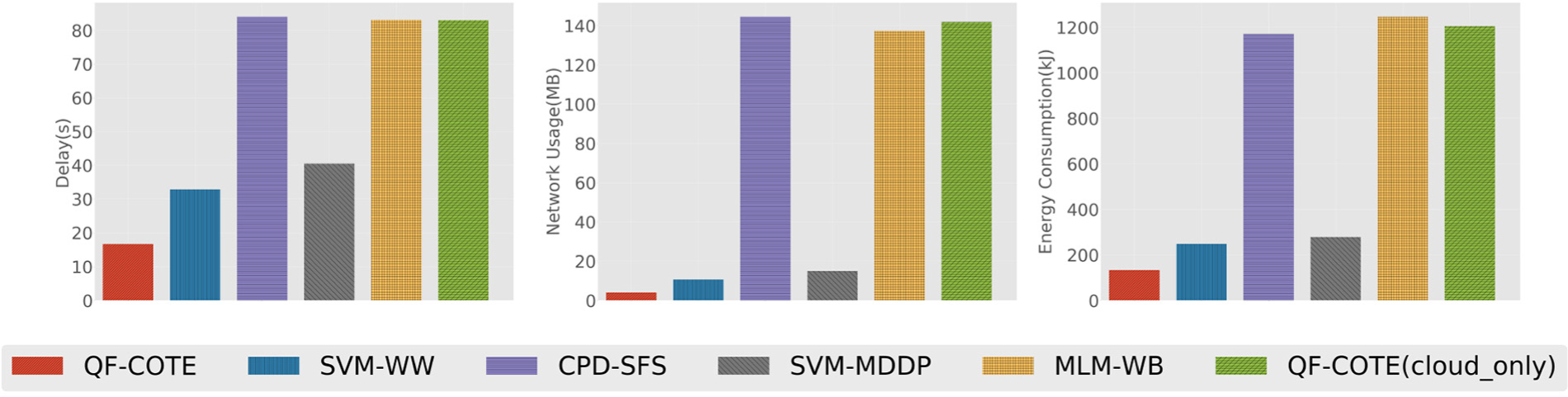
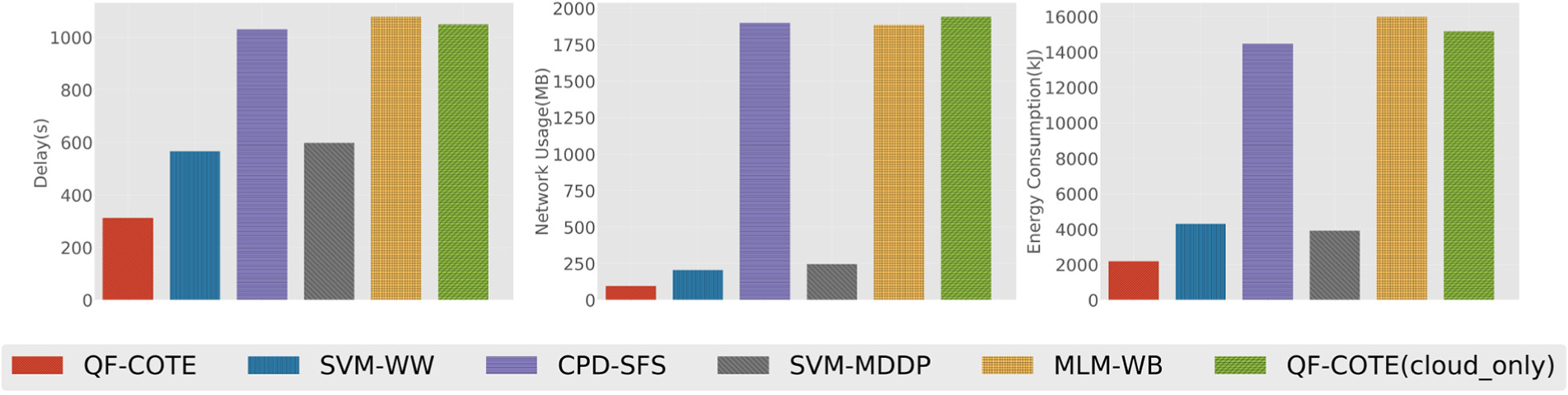
Performance of different methods in simulation based on data set 2.

For these existing methods, SVM-WW and SVM-MDDP support data preprocessing, while CPD-SFS and MLM-WB do not.

From the four figures, we can observe that (1) the methods that utilize data preprocessing perform better than those do not. In both data sets, methods with edge computing procedure will cost about half time and about 1/10 network resource to transfer the message. For the respective energy consumption, the former cost less than one-fourth than the latter. (2) Our method performs less than half of the best existing method, which is SVM-WW. First, our method detect a flexible length threshold window instead of a fixed length window, making the network consumption decrease. Second, random forest algorithm is more efficient than SVM-WW’s method in the phone. Last but not the least, the main algorithm COTE is much more efficient, which leads to a less delay. (3) In a bigger data set, the ratio between the cloud computing methods and edge computing methods decreases, which indicates that these methods are more suitable for the data size less than 100 or 1000 GB. Under this scale of data, our method still possesses advantages.

Performance with different velocity and sample frequency

Influence of different velocity

As it can be seen in Figure 13, the F1 score first rises as the speed of the car increases and then start falling after a certain speed value. It can be explained that with the increase in the speed, the collision between the vehicle and the anomaly becomes more severe, causing more information in one anomaly window. The characteristics of anomalies become more apparent as the amount of information increases. However, the time spent on the same length of anomaly will gradually become shorter, which means the anomaly window detected by the model decreases as the speed increases. A too short window makes a lot of information directly ignored, which reduces the recognition effect. For our model, F1 score reaches climax with the speed of 80, 40, and 60, respectively, and the average F1 score reaches the best with the speed of 60. This speed is close to the normal speed of the vehicle. As a result, our model can be applied to most vehicle in the case of edge computing, thus our model is fit for widely detecting road anomalies.

Figure 13.

Influence of velocity to our proposed method.

Influence of different sample frequency

As it can be seen in Figure 14, the F1 score first rises rapidly as the frequency increases and then start falling slowly after a certain frequency. It can be explained that in a low sample frequency, the data point increases rapidly from 10 to 20 and 20 to 30. As a result, there will be more information in one anomaly window. The characteristics of anomalies become more apparent as the amount of information increases. For our method, it will transform anomaly windows with different length into the same length, normally into the shortest length. The information losses during the change. With the increase in sample frequency, the difference in the shortest length and the average length of window anomaly will increase as well, which causes more loss in information. Thus, the F1 score decreases slowly over the sample frequency of 120. As a result, the sample rate in our model should be set in an appropriate value to avoid the loss.

Figure 14.

Influence of sample rate to our proposed method.

Conclusion

Smartphones are becoming easier to use as data collection devices, making it more possible to analyze road conditions with these data. In this work, we propose a model to detect the anomaly on the road based on a series of acceleration data. We first analyze the theoretical possibility of threshold detection and the random forest filter and then apply COTE to these time windows to define the anomaly type. We test our method in two data sets using F1 score as the metric to compare to some existing methods. Our method takes much advantage over all the other methods in two data sets, indicating that the model is usable in most situations. In addition, we simulate edge computing situations and the results prove that our method is more suitable for the edge computing situation. We take far less time, energy, and network consumption compared to the best existing method, which means we only use half of the resource that the best existing method needs to reach a better performance.

In the future work, we would like to apply this system to a large amount of taxies and generate a map of the entire anomalies in the city with group perception. It requires the judgment and selection of the large amount of data and will help the government to repair the road in a more simple way.

Footnotes

Handling Editor: Rodolfo Meneguette

Declaration of conflicting interests

The author(s) declared no potential conflicts of interest with respect to the research, authorship, and/or publication of this article.

Funding

The author(s) disclosed receipt of the following financial support for the research, authorship, and/or publication of this article: This work is supported by the Young Scientists Fund of the National Natural Science Foundation of China (Grant No. 61802343), Zhejiang Provincial Natural Science Foundation of China (Grant No. LGF19F020019), and Hangzhou Key Laboratory for IoT Technology & Application.

ORCID iD

Mingxuan Zhou

References

Seraj

Meratnia

Havinga

. RoVi: continuous transport infrastructure monitoring framework for preventive maintenance. In: 2017 IEEE international conference on pervasive computing and communications (PerCom), Kona, HI, 13–17 March 2017, pp.217–226. New York: IEEE.

Carlos

Aragn

Gonzclez

, et al. Evaluation of detection approaches for road anomalies based on accelerometer readings—addressing who’s who. IEEE T Intell Transp 2018; 19: 3334–3343.

Mohan

Padmanabhan

Ramjee

. Nericell: rich monitoring of road and traffic conditions using mobile smartphones. In: Proceedings of the 6th ACM conference on embedded network sensor systems (SenSys ’08), Raleigh, NC, 5–7 November 2008, pp.323–336. New York: ACM.

Mednis

Strazdins

Liepins

, et al. RoadMic: road surface monitoring using vehicular sensor networks with microphones. In: International conference on networked digital technologies, Prague, 7–9 July 2010, pp.417–429. Berlin, Heidelberg: Springer.

Wahlstrm

Skog

Händel

. Smartphone–based vehicle telematics: a ten-year anniversary. IEEE T Intell Transp 2017; 18(10): 2802–2825.

Eriksson

Girod

Hull

, et al. The pothole patrol: using a mobile sensor network for road surface monitoring. In: Proceedings of the 6th international conference on mobile systems, applications, and services (MobiSys ’08), Breckenridge, CO, 17–20 June 2008, pp.29–39. New York: ACM.

Mednis

Strazdins

Zviedris

, et al. Real time pothole detection using android smartphones with accelerometers. In: 2011 international conference on distributed computing in sensor systems and workshops (DCOSS), Barcelona, 27–29 June 2011, pp.1–6. New York: IEEE.

Perttunen

Mazhelis

Cong

, et al. Distributed road surface condition monitoring using mobile phones. In: Proceedings of the 8th international conference on ubiquitous intelligence and computing (UIC ‘11), Banff, AB, Canada, 2–4 September 2011. Berlin, Heidelberg: Springer-Verlag.

Seraj

van der Zwaag

Dilo

, et al. RoADS: a road pavement monitoring system for anomaly detection using smart phones. In: Atzmueller

Chin

Janssen

, et al. (eds) Big data analytics in the social and ubiquitous context. Cham: Springer International Publishing, 2016, pp.128–146.

10.

Carlos

Gonzalez

Martinez

, et al. Evaluating reorientation strategies for accelerometer data from smartphones for its applications. In: Garcia

Caballero-Gil

Burmester

, et al. (eds) Ubiquitous computing and ambient intelligence. Cham: Springer International Publishing, 2016, pp.407–418.

11.

El-Wakeel

Noureldin

, et al. Towards a practical crowdsensing system for road surface conditions monitoring. IEEE Internet Things Journal 2018; 5: 4672–4685.

12.

González

Moreno

Escalante

, et al. Learning roadway surface disruption patterns using the bag of words representation. IEEE T Intell Transp 2017; 18(11): 2916–2928.

13.

Cong

Hautakangas

Nieminen

, et al. Applying wavelet packet decomposition and one-class support vector machine on vehicle acceleration traces for road anomaly detection. In: Guo

Hou

Zeng

. (eds) Advances in neural networks—ISNN 2013. Berlin, Heidelberg: Springer, 2013, pp.291–299.

14.

El-Wakeel

Rahman

, et al. Monitoring road surface anomalies towards dynamic road mapping for future smart cities. In: 2017 IEEE global conference on signal and information processing (GlobalSIP), Montreal, QC, Canada, 14–16 November 2017, pp.828–832. New York: IEEE.

15.

Gia

Jiang

Rahmani

, et al. Fog computing in healthcare internet of things: a case study on ECG feature extraction. In: 2015 IEEE international conference on computer and information technology; ubiquitous computing and communications; dependable, autonomic and secure computing; pervasive intelligence and computing, Liverpool, 26–28 October 2015, pp.356–363. New York: IEEE.

16.

GuArout

Monteil

Costa

, et al. Energy-aware simulation with DVFS. Simul Model Pract Th 2013; 39: 76–91.

17.

Liu

, et al. Smartroad: smartphone-based crowd sensing for traffic regulator detection and identiﬁcation. ACM Trans Sen Netw 2015; 11(4): 551–5527.

18.

Fox

Vijaya Kumar

BVK

Bai

Multi-source variable-rate sampled signal reconstructions in vehicular CPS. In: IEEE INFOCOM 2016—the 35th annual IEEE international conference on computer communications, San Francisco, CA, 10–14 April 2016, pp.1–9. New York: IEEE.

19.

Fox

Vijaya Kumar

BVK

Chen

, et al. Multi-lane pothole detection from crowdsourced undersampled vehicle sensor data. IEEE T Mobile Comput 2017; 16(12): 3417–3430.

20.

Xue

Zhu

, et al. Pothole in the dark: perceiving pothole profiles with participatory urban vehicles. IEEE T Mobile Comput 2017; 16(5): 1408–1419.

21.

Alessandroni

Carini

Lattanzi

, et al. A study on the influence of speed on road roughness sensing: the smartroadsense case. Sensors 2017; 17(2): E305.

22.

Seraj

Havinga

PJM

Meratnia

SpinSafe: an unsupervised smartphone-based wheelchair path monitoring system. In: 2016 IEEE international conference on pervasive computing and communication workshops (PerCom Workshops), Sydney, NSW, Australia, 14–18 March 2016, pp.1–6. New York: IEEE.

23.

Madli

Hebbar

Pattar

, et al. Automatic detection and notification of potholes and humps on roads to aid drivers. IEEE Sens J 2015; 15(8): 4313–4318.

24.

Harikrishnan

Gopi

. Vehicle vibration signal processing for road surface monitoring. IEEE Sens J 2017; 17(16): 5192–5197.

25.

Chuang

Nian

. Toward crowdsourcing-based road pavement monitoring by mobile sensing technologies. IEEE T Intell Transp 2015; 16(4): 1905–1917.

26.

Bagnall

Lines

Hills

, et al. Time-series classification with cote: the collective of transformation-based ensembles. IEEE T Knowl Data En 2015; 27(9): 2522–2535.

27.

Allouch

Koubaa

Abbes

, et al. RoadSense: smartphone application to estimate road conditions using accelerometer and gyroscope. IEEE Sens J 2017; 17(13): 4231–4238.

28.

El-Wakeel

Osman

Noureldin

, et al. Road test experiments and statistical analysis for real-time monitoring of road surface conditions. In: GLOBECOM 2017 – 2017 IEEE global communications conference, Singapore, 4–8 December 2017, pp.1–6. New York: IEEE.

29.

Fox

Vijaya Kumar

BVK

Chen

, et al. Crowdsourcing undersampled vehicular sensor data for pothole detection. In: 2015 12th annual IEEE international conference on sensing, communication, and networking (SECON), Seattle, WA, 22–25 June 2015, pp.515–523. New York: IEEE.

30.

Gupta

Dastjerdi

Ghosh

, et al. iFogSim: a toolkit for modeling and simulation of resource management techniques in internet of things, edge and fog computing environments. J Softw: Prac Exp 2017; 47: 1275–1296.

Enabling real-time road anomaly detection via mobile edge computing

Abstract

Keywords

Introduction

Related work

Overview of the proposed design

Design framework

Threshold detection and sliding window processing

A Quick filter of the normal window and the abnormal window

Using COTE to determine the type of anomalies

Experiment evaluation

Experimental settings

Data sets

Comparative methods

Evaluation metric

Identification performance for all methods

Edge computing performance for all methods

Hardware environment

Consumption analysis

Performance with different velocity and sample frequency

Influence of different velocity

Influence of different sample frequency

Conclusion

Footnotes

Declaration of conflicting interests

Funding

ORCID iD

References