Sage Journals: Discover world-class research

Abstract

The running state of a geared transmission system affects the stability and reliability of the whole mechanical system. It will greatly reduce the maintenance cost of a mechanical system to identify the faulty state of the geared transmission system. Based on the measured gear fault vibration signals and the deep learning theory, four fault diagnosis neural network models including fast Fourier transform–deep belief network model, wavelet transform–convolutional neural network model, Hilbert-Huang transform–convolutional neural network model, and comprehensive deep neural network model are developed and trained respectively. The results show that the gear fault diagnosis method based on deep learning theory can effectively identify various gear faults under real test conditions. The comprehensive deep neural network model is the most effective one in gear fault recognition.

Keywords

Fault diagnosis gear vibration signal processing neural network deep learning

Introduction

Gears are widely used in transportation, mechanical processing, aerospace, power system, agricultural mechanized production, and other modern industries. Due to its long-term continuous operation, poor working environment, and other reasons, the geared transmission system is prone to damage and failure. In the transmission systems, 80% of the faults are caused by gears, which will significantly affect the safety and reliability of equipment. Therefore, identification of gear system faults will greatly improve the reliability of the mechanical system and reduce accidents caused by gear faults. As shown in Figure 1, fault diagnosis usually consists of four steps: signal collection, feature extraction (signal processing), state recognition, and diagnosis and decision.

Figure 1.

Fault diagnosis process.

When the gearbox is malfunctioning, the energy distribution and frequency components of the vibration signal are abnormal. Therefore, the extraction of parameters that are sensitive to faults, such as frequency components and the amplitude changes, can provide valuable information for fault diagnosis. Vibration analysis has become the most effective and widely used method of gearbox faults diagnosis, because of its advantages such as fast speed, high precision, accurate fault locating, and online diagnosis.

The process of vibration signal processing is to separate the characteristic signal related to the fault from the vibration signal, and to judge the faults of the mechanical system by analyzing the separated signal. At present, the signal processing technology in the mechanical fault diagnosis can be divided into two categories: one is the traditional mathematical processing method represented by the fast Fourier transform (FFT), and the other is the intelligent diagnosis technology represented by the neural network. Traditional mathematical processing methods mainly include linear stationary mathematical transformation methods and non-stationary, non-Gaussian distribution and nonlinear random signal processing methods. The linear stationary mathematical transformation methods are represented by time domain statistical analysis,¹ frequency domain statistical analysis,² Fourier transform analysis,³ time series model analysis method,⁴ refined spectrum analysis,⁵ holographic spectrum analysis,⁶ singular spectrum noise reduction method,⁷ matching tracking analysis,⁸ and geometric fractal analysis method.⁹ Non-stationary, non-Gaussian distribution, and nonlinear random signal processing methods are represented by high-order spectral analysis,¹⁰ principal component analysis,¹¹ short-time Fourier transform (STFT),¹² Wigner–Ville distributing,¹³ wavelet transform (WT),¹⁴ cyclic stationary analysis method,¹⁵ random resonance method,¹⁶ empirical mode decomposition (EMD),¹⁷ Hilbert–Huang transform (HHT),¹⁸ and the second-generation WT method.¹⁹ Intelligent diagnosis technology methods mainly include intelligent diagnosis technology based on an expert system,²⁰ intelligent diagnosis technology based on an artificial neural network,²¹ intelligent diagnosis technology based on a fuzzy logic,²² intelligent diagnosis technology based on a genetic algorithm,²³ fault diagnosis technology based on a fuzzy neural network,²⁴ and so on.

In traditional fault diagnosis, it is difficult to establish an effective fault diagnosis database. For the traditional mathematical transformation method, it shows poor robustness to noise, and there should be a lot of engineering practice experience as auxiliary supports, which are the main limits. The main disadvantages of intelligent diagnosis technology are its low efficiency and accuracy. Therefore, it is necessary to develop a reliable fault diagnosis method that can effectively identify and extract fault features, and replace the current identification method which relies on a lot of existing engineering experience, so as to realize the development and breakthrough of geared system fault diagnosis technology.

Recently, more and more studies of the mechanical system fault diagnosis focused on the theory of deep learning, whose essence is to deeply extract the characteristic information in the data. Huang et al.²⁵ developed a fault diagnosis method of vehicle suspension vibration isolator based on a deep belief network (DBN). Lei et al.²⁶ applied the deep learning theory to the fault diagnosis of a gear system. Zhao et al.²⁷ applied DBN to study the fault identification of bearing. Lu et al.²⁸ used stacked denoising autoencoder to identify bearing faults and achieved good results. Cao et al.²⁹ proposed a deep convolutional neural network (CNN)–based transfer learning method to diagnose gear faults, and this method was robust even with a few training data. Chen et al.³⁰ adopted a multi-layer neural networks–based DBN to diagnose gear faults, in which multidimensional feature sets were used. Zeng et al.³¹ combined the S-transform and CNN to implement gear faults diagnosis and found that CNN had a higher classification rate and less computing time than DBN and stacked autoencoder. Li et al.³² introduced an augmented deep sparse autoencoder approach to effectively diagnose the gear wear and pitting faults with a few raw vibration data. He et al.³³ proposed a deep believe network–based artificial intelligence approach which used the unlabelled time domain data to perform gear faults diagnosis. Wang et al.³⁴ demonstrated that the frequency domain features outperformed the time domain features for gear faults diagnosis. Heydarzadeh et al.³⁵ developed different deep neural networks for vibration, acoustic, and torque signals, and the discrete WT data were used to extract gear faults feature. Li et al.³⁶ used the preprocessing current signals to detect faults in a planetary gear set under different conditions.

In this article, the faulty gear vibration test bench is built and the fault vibration signal is extracted. Based on the deep learning theory, the FFT, CWT (continuous wavelet transform), and HHT of vibration signal and the combination of the three signals are used as input, and the deep learning neural network models for gear fault diagnosis are developed and trained.

Vibration test of gear fault

The deep learning network needs enough gear fault signals as training and test samples. In order to obtain the vibration signal of gear system under different fault conditions, gears with different faults are designed and manufactured, and a back-to-back gear vibration test rig is built. The injection mode of each gear fault is single-gear and single-tooth fault; that is, each fault only occurs in a single-gear tooth of a single gear. The vibration acceleration signals of the single-stage geared transmission system are tested. Detailed description of the whole system and related parameters are as follows.

Fault injections of gears

Single-stage spur gears are used here. The basic parameters of gears are shown in Table 1. The photograph of normal gears is shown in Figure 2.

Table 1.

Basic gear parameters.

	Teeth number	Normal module	Pressure angle	Helix angle	Face width	Modification coefficient	Quality grade
Pinion	16	4.5 mm	20°	0°	20 mm	0.85	6
Wheel	24	4.5 mm	20°	0°	20 mm	−0.5	6

Figure 2.

Photograph of normal gears.

Gear faults and operational states used in this article are shown in Table 2. Gear faults are only injected into the wheel not the pinion, and four kinds of fault are adopted.

Table 2.

Gear faults and operational states.

States	0	1	2	3	4
Pinion	Normal	Normal	Normal	Normal	Normal
Wheel	Normal	Tooth wear	Tooth broken	Gear crack	Tooth pitting

Figure 3 shows the photograph of faulty gears. Each gear fault is a single-tooth fault; that is, all gear faults only occur in a single-gear tooth.

Figure 3.

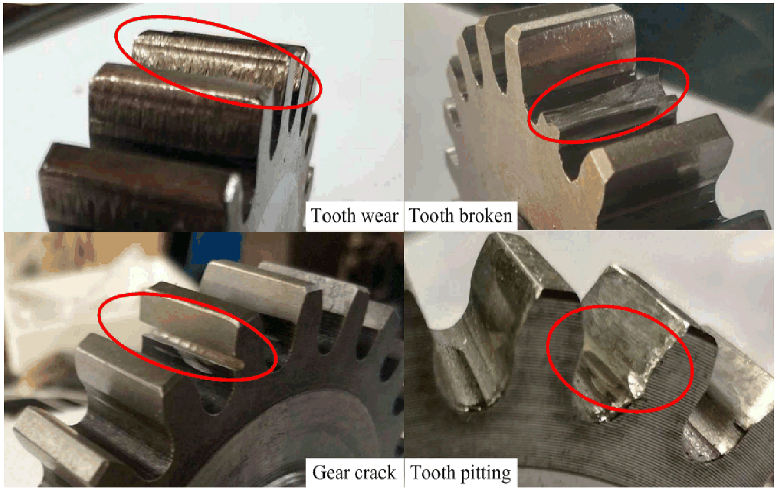
Photograph of gear faults.

Layout and basic parameters of the test rig

The test rig is a back-to-back gear system, as shown in Figure 4. It is mainly composed of an electric motor, test gearbox, slave gearbox, and loading unit. Among them, the test gearbox is the core unit of this test rig. All gears in different states described above will be used in this gearbox.

Figure 4.

Photograph of the back-to-back test rig.

The motor used in this test is a three-phase AC asynchronous motor, and the speed regulation mode is AC frequency conversion. In this experiment, the motor speed is 1495 r/min, and a 150N•m fixed torque is added to the pinion by the loading coupling. By combining with the gear parameters, the basic vibration parameters of the test rig can be obtained, which are shown in Table 3.

Table 3.

Basic vibration parameters of the test rig.

Z ₁	Z ₂	n ₂	f_z	f_n ₁	f_n ₂
16	24	1495 r/min	598 Hz	34.4 Hz	24.9 Hz

In Table 3, Z₁ is the number of pinion teeth, Z₂ is the number of wheel teeth, n₂ is the rotational speed of the wheel, f_z = z₁ × n₁/60 = 598 Hz is the meshing frequency of the geared transmission system, and f_n₂ = n₂/60 = 24.9 Hz and f_n₁ = n₁/60 = 37.4 Hz are the shaft frequencies.

Gear vibration test systems

The vibration test system consists of an accelerometer and a data acquisition system. The accelerometer is mainly used to collect vibration acceleration signals of gearbox and convert them into the charge signals. The accelerometer used in this article is PCB333B40 produced by PCB company, with one direction and a sensitivity of 500 mV/g. The main functions of the data acquisition system are to collect, amplify, and transfer the charge signals output by the accelerometer to the data collection software. The data acquisition system selected for this test is the eight-channel data acquisition analyzer Mi-7008 of Econ company.

The measuring points of the sensor are shown in Figure 5. Figure 5(a) is the schematic diagram of accelerometer locations, and the vibration detection direction of each sensor is indicated by the arrow on the sensor. Figure 5(b) is the corresponding photograph.

Figure 5.

Sensor layout: (a) sketch and (b) photograph.

Data acquisition and pretreatment

Vibration data acquisition of faulty gear

The purpose of the experiment is to collect enough vibration signal samples of gears under different operating conditions, so as to provide data sources for subsequent neural network training and prediction. The sample number of each failure in this test is 900. The gear vibration signals of several mesh periods are collected, and the sampling time taken in this test is 1 s. In order to simplify the operation, the sampling time of each failure mode in this test is taken as 30 min, and the number of final samples should be 30×60=1800. To further increase the randomness, 900 samples are randomly selected from the original 1800 ones as the final test samples. Since the mesh frequency of the test gear is 598 Hz, the sampling frequency f_s of the accelerometer should be at least twice of the mesh frequency, that is, f_s = 2f_z = 1196 Hz, and 2048 Hz is used in this test.

Figures 6(a)–(c) are vibration data collected by no. 1, no. 2, and no. 3 sensors, respectively. It can be seen from the test data that the real gear vibration signals are not regular, and there are many shocks or even irregular drift due to gear faults.

Figure 6.

Vibration acceleration signal: (a) channel 1, (b) channel 2, and (c) channel 3.

Signals of different channels can reflect vibrations of different locations and directions. The gear fault features may not appear in the vibration signals of some measurement points, or the faulty features of some single point may be submerged by noise, which will worsen the fault diagnosis results. If the vibration signals from three channels are simply stacked, the computation efficiency of the deep learning network will be significantly reduced. In order to comprehensively consider the vibration signals of the three channels and reduce the computation cost of the deep learning network, composite vibration acceleration is used, as shown in equation (1). Different signals are synchronously collected to ensure they are aligned with time. Figure 7 is the composite vibration acceleration, which reflects the overall vibration of the gearbox to some extent, while the direction and phase information are lost

a_{c} (t) = \sqrt{a_{1}^{2} (t) + a_{2}^{2} (t) + a_{3}^{2} (t)}

(1)

Figure 7.

Composite vibration acceleration signal.

where a_c is the composite vibration acceleration, a₁ is the vibration acceleration of channel 1, a₂ is the acceleration of channel 2, and a₃ is the vibration acceleration of channel 3.

Sample and segmentation of original test data

The original experimental data are five sets of data under five operating states, and each data set with a data volume of 1800. All samples of each data set are in the same running state, and 900 samples are randomly selected from the original 1800 ones to serve as the final experimental samples.

To complete the training and test for the neural network, the original data need to be randomly sorted and composed into a sample set of 4500 samples. Then, 500 samples are selected from the sample set with a sample size of 4500 as the test samples of the network, and the remaining 4000 samples are the training samples of the network. In this way, the original training and test sample sets are obtained.

Traditional mathematical transformations of sample data

The input data sources of the deep learning model in this article are FFT, WT, and HHT signals of gear vibration. Thus, it is necessary to carry out corresponding mathematical transformation for the original vibration acceleration signal samples.

FFT

FFT is an ideal method to quickly convert discrete time domain signals into frequency domain signals. It gets a powerful ability to identify stationary periodic signals, and it can recognize signals whether they are amplitude modulated or frequency modulated. However, if a frequency component does not have a complete period in the observation area, or there is a frequency component changing with time in the signal, the FFT cannot analyze the measured signals accurately.

The mathematical basis of FFT is Fourier transform (FT), and the formula of FT is

F (ω) = \int_{- \infty}^{\infty} f (t) e^{- j ω t} dt

(2)

where $F (ω)$ is the converted signal function in the frequency domain, $ω$ is the independent variable of the frequency domain function, namely the signal frequency, and $f (t)$ is the time domain signal function to be converted.

Figures 8(a)–(c) are FFT of acceleration signals of no. 1, no. 2, and no. 3 accelerometers, respectively. Figure 9 is the FFT of the composite vibration acceleration signals. It can be seen from each FFT figure that the vibration acceleration signals collected by channel 2 are the closest to the theoretical gear meshing vibration spectrum, and the composite channel can reflect the theoretical vibration spectrum of meshing gear well.

Figure 8.

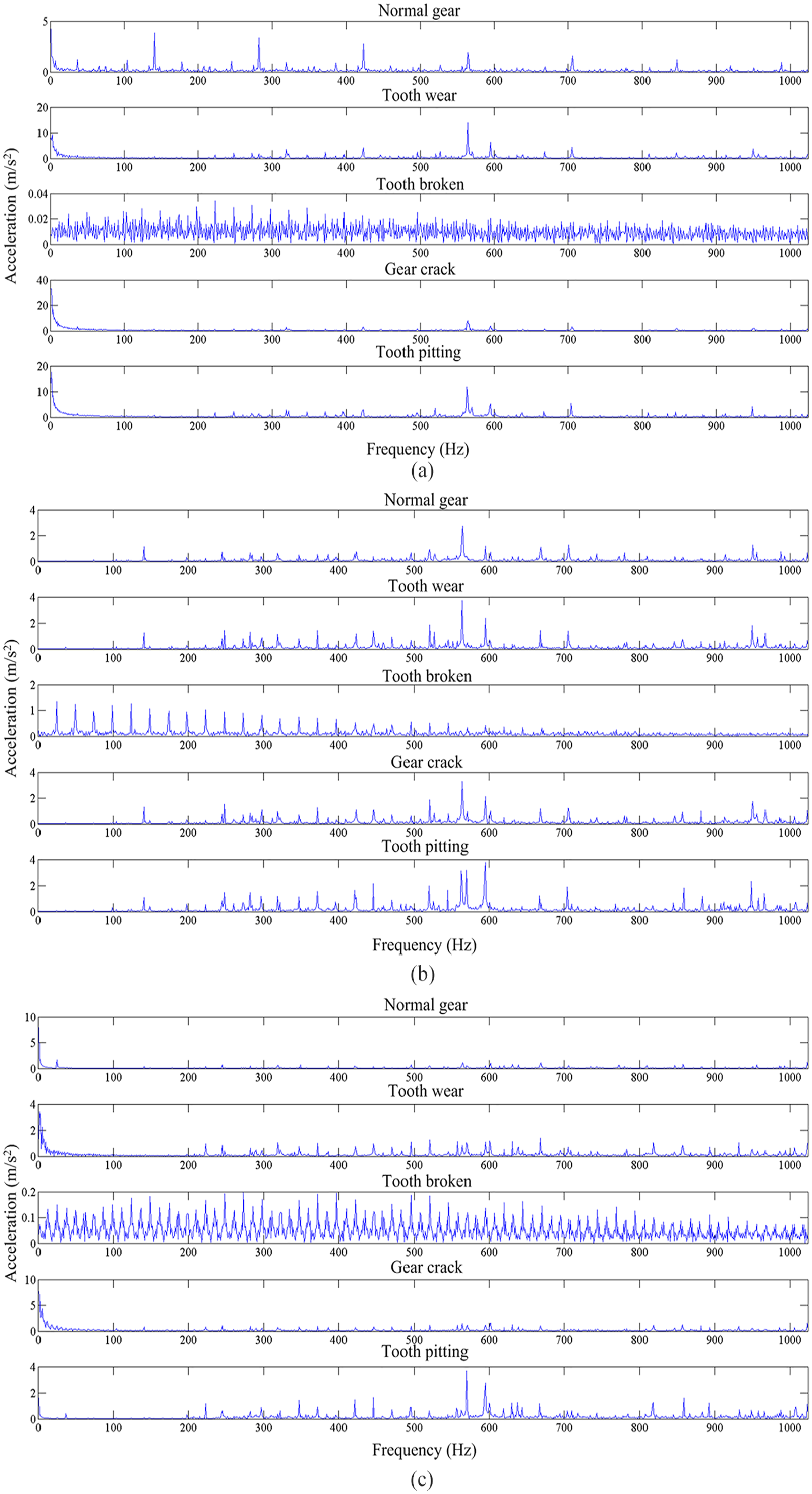
FFT of acceleration signal of each channel: (a) channel 1, (b) channel 2, and (c) channel 3.

Figure 9.

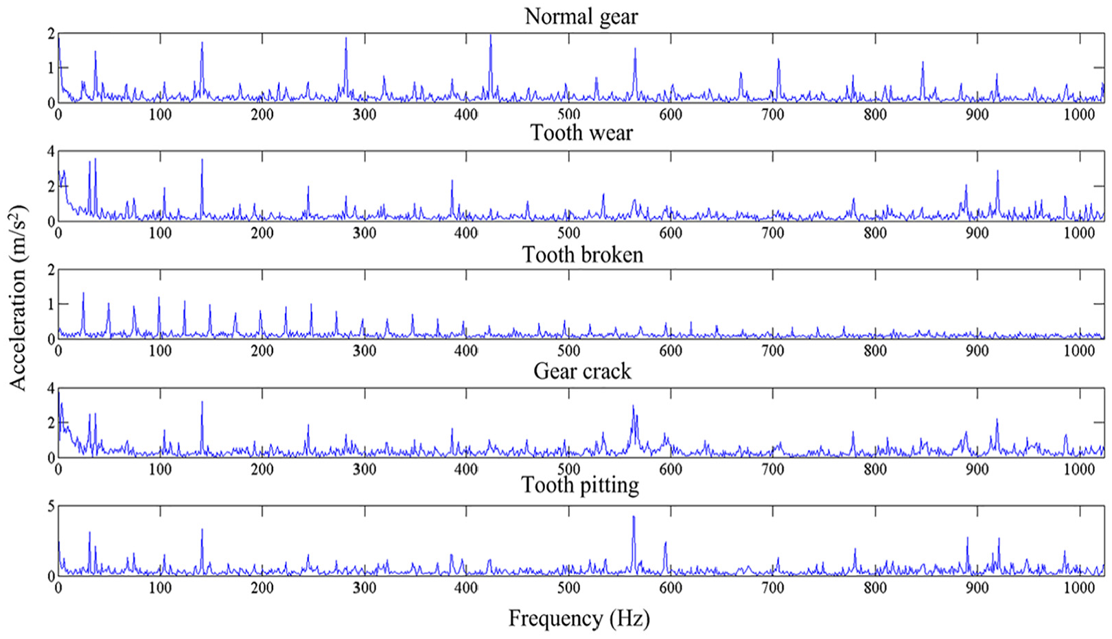
FFT of composite acceleration signal.

WT

The WT is different from the FFT, and it does not take the fixed sinusoidal wave basis as the transform basis of the signal. In a sense, the WT is similar to the STFT. On the one hand, by adding small windows to the signal waves in the time domain, the average signal transform in the signal window can be obtained, so as to form the time spectrum of the whole signal in the time domain. On the other hand, WT uses the wavelet base instead of the sinusoidal wave base that smoothly varies with time, which can overcome the energy loss of STFT caused by window. As a result, WT makes the whole signal spectrogram tends to smooth, which could be used to analyze the signal accurately. Although WT is the most widely used method for time-frequency analysis of signals, it is affected by the law of uncertainty. WT is also unable to accurately measure the data both in frequency and time domains at the same time.

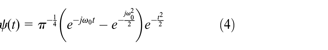
The mathematical transformation expression of WT is

WT (a, τ) = \frac{1}{\sqrt{a}} \int_{- \infty}^{\infty} f (t) \cdot ψ (\frac{t - τ}{a}) dt

(3)

where $a$ is the scale parameter, which controls the scaling of wavelet basis, $τ$ is the translation parameter, which controls the delays of wavelet basis, $ψ (t)$ is the wavelet basis or the generating wave, and Morlet wavelet basis function is used here

ψ (t) = π^{- \frac{1}{4}} (e^{- j ω_{0} t} - e^{- \frac{j ω_{0}^{2}}{2}}) e^{- \frac{t^{2}}{2}}

(4)

where $ω_{0}$ is the central frequency of the wavelet basis of Morlet.

Figure 10 shows the WT time–frequency spectrum of acceleration signals of no. 1, no. 2, and no. 3 accelerometers. It can be seen that the time–frequency spectrum of channel 2 is the closest to the vibration signal of the theoretical meshing gear, and there is a peak at about 600 Hz, which is basically in line with the theoretical mesh frequency of 598 Hz.

Figure 10.

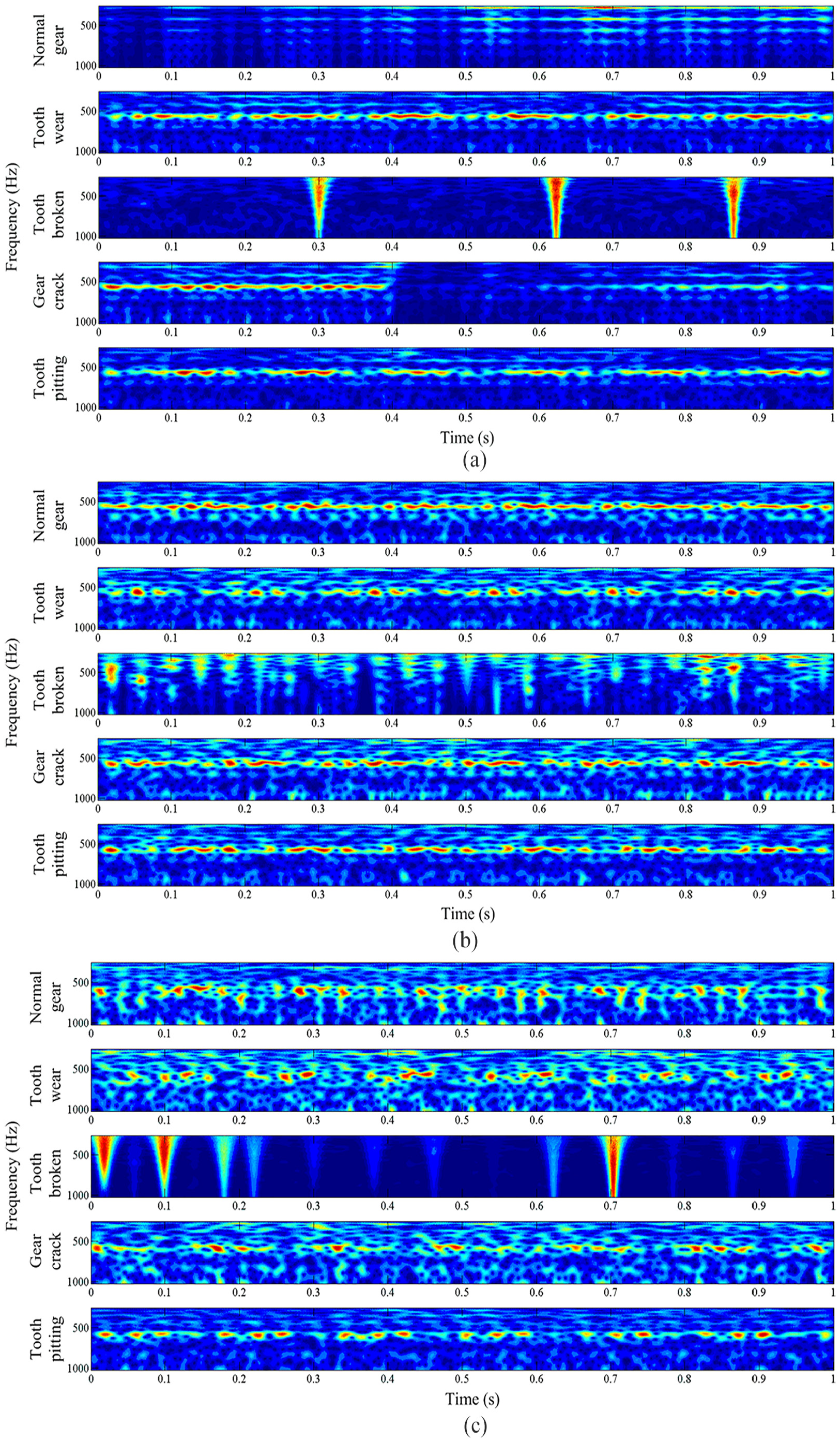
WT spectrum of vibration acceleration signal: (a) channel 1, (b) channel 2, and (c) channel 3.

Hilbert–Huang transformation

HHT is a typical signal adaptive analysis method. This method is based on EMD combined with Hilbert spectrum in Hilbert transform (HT) and its spectral analysis method. It is suitable for non-steady state, nonlinear signal analysis. Due to the existence of EMD, this kind of transformation is different from the traditional transformation mode using fixed fundamental wave or fixed conversion formula, and it gets a powerful ability to analyze the measured signal spectrum. HHT mainly includes two transformation links, which are EMD and Hilbert transform. The HHT spectrum can be used to analyze complex non-stationary and nonlinear signals, which can be obtained by these two links. However, even with the improved EMD, there is still some instability in the process of signal decomposition, and there is also the possibility that the decomposed signals may be confused with each other, making the Hilbert transform invalid. Therefore, the identification of the HHT also has some limitations.

Figure 11 shows the HHT energy spectrum of vibration acceleration signals of no. 1, no. 2, and no. 3 accelerometers.

Figure 11.

HHT energy spectrum of vibration acceleration signal: (a) channel 1, (b) channel 2, and (c) channel 3.

Signal normalizations and spectrum compression

The output signal of the above three kinds of mathematical transformation method is not normalized, and the neural network’s activation function is a typical kind of nonlinear saturation function. If the value of the input data is too big or too small, it will cause the corresponding error gradient saturates or disappears. Thus, the input signal in the network should be normalized. In view of these, the mathematical transformation of the signal should be normalized.

For WT and HHT, the final results are both two-dimensional matrices. The size of a WT matrix is 768 × 2048. If it is calculated with the original dimension, each matrix will cost 12 MB of system memory, and 900 matrices will approximately occupy 11 GB. Besides, HHT (the matrix size is 400 × 2048) costs about 6 GB of memory. The storage and computing of such a large amount of data are really great challenges, so the data must be cut out and compressed.

From Figures 10 and 11, it can be seen that the vibration signals of the gear show periodic fluctuations, so it only needs to intercept the signals within one or two operating cycles. Since the frequency of the faulty gear is 24.9 Hz, the WT signals from 0 to 0.1 s are taken as the input signals of the neural network. The size of the final compressed wavelet time–frequency spectrum is 768 × 204. The HHT signal is also compressed, and the final energy spectrum size is 400 × 410.

Establishment and implementation of deep learning model

After the transformation and processing of the original vibration signals mentioned above, the original vibration signals have been transformed into a sample data set that can be input into each deep learning model for effective training and testing. The FFT-DBN model, WT-CNN model, HHT-CNN model, and the Co-NN (composite neural network) model will be established.

Establishment and training of FFT-DBN

The deep confidence network (DBN) gets powerful identification ability for discrete one-dimensional signals, while it cannot perfectly hold the dimensional information about multi-dimension input signals. At the same time, the DBN is a typical fully connected network, which inconveniences the training of long signals and significantly decreases the fault diagnosis capability. Due to the limitation of the computational performance of the DBN and the computational capacity of the computer, it is not possible to effectively establish the DBN considering all channel signals at the same time. Therefore, the composite channel signal is used to roughly replace the vibration signals networks of the three channels. There are four sets of FFT sample sets, namely channel 1, channel 2, channel 3, and the composite channel. Based on these four signal sample sets, four FFT-DBNs are established and trained respectively.

The network structure is shown in Figure 12, which is stacked by multi-layer restricted Boltzmann machines. The dimension of the FFT data obtained in this experiment is 1024 rows, so there are 1024 neurons in the input layer of the network. The output of the lower restricted Boltzmann machine serves as the input of the neighbor upper layer, thus forming the ith hidden layer. There are three hidden layers in this DBN, and the numbers of neurons are 512, 256, and 128, respectively. Finally, after the Nth hidden layer, a multinomial logistic regression (also known as softmax) is constructed as the final nonlinear classifier of the network. The final sample classification number is 5, so the final neurons number in the output layer is 5.

Figure 12.

Diagram of DBN.

The sample batch value is 20, and the number of sampling iterations is 200. The errors in the training process of the four DBNs are shown in Figure 13. The training results of channel 2 are the most ideal, which is also consistent with the results mentioned in the previous paper that the spectrum of channel 2 is the closest to the theoretical spectrum. Finally, the training accuracy of no. 1, no. 2, no. 3, and the composite channel are 71%, 86%, 70% and 78%, respectively. Sample testing accuracy of no. 1, no. 2, no. 3, and the composite channel are 62.4%, 83.2%, 66.4%, and 70.2%, respectively, as shown in Figure 14.

Figure 13.

Training error rate variation diagram of the FFT-DBN.

Figure 14.

Testing accuracy rate of the FFT-DBN.

By the comparison of the training errors and testing accuracy between different channels, it can be seen that the channel 2–based DBN has the best gear fault identification ability. The composite channel signal no more effectively reflects the gear faults; instead, it has weakened the signal characteristics of channel 2.

Establishment and training of WT-CNN and HHT-CNN

The output signals of WT and HHT used in this article for fault features extraction are both two-dimensional data. CNN gets a powerful learning ability to two-dimensional correlated signals than other networks. It is a typical non-fully connected neural network which has an excellent robustness and low training difficulty. Due to its distributed multi-channel parallel computing, the CNN has a higher training speed than most one-dimensional fully connected networks. Different from the DBN, CNN itself can be multi-channel data input. Therefore, the acceleration signals of the three measurement points acquired in this experiment can be directly input into the network through three different input channels; that is, CNN established in this article is a neural network under multi-channel input.

As shown in Figure 15, WT-CNN has a three-layer convolutional network structure. The pooling layer of the first convolutional network uses non-equal values of row and column sliding windows, while the other layers use equivalent manner for the row and column sliding windows. The input data are three 768 × 204 matrices, which are converted into three hundred eighty-four 10 × 5 matrices after three times of convolution pooling operation, which are then transformed into the final five gear fault states after three layers of logistic regression neural network processing.

Figure 15.

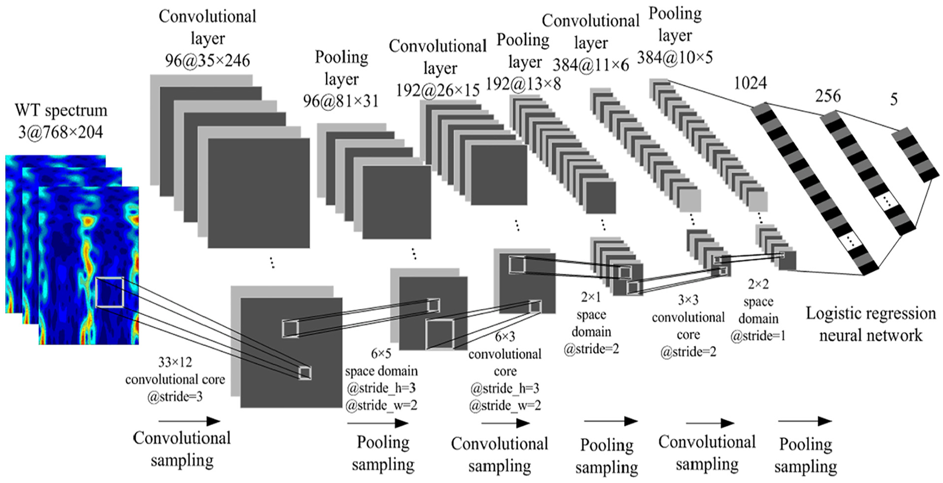
Structure of WT-CNN under three-channel input.

HHT-CNN is shown in Figure 16. The input signals are the HHT of vibration acceleration under three channels, which are three matrices with a dimension of 400 × 410. A CNN network which contains three-layer convolutional networks (the convolutional network has one convolutional layer and one pooling layer) and three-layer logistic regression networks is used to diagnose the gear fault. Input HHT data are converted into 384 matrices of 5 × 5 size through the three-layer convolutional network structure. Then, the data are converted into 1 row 1024 columns after the one dimension sequence processing, and finally converted into five gear fault states through the logistic regression neural network.

Figure 16.

Structure of HHT-CNN under three-channel input.

The training methods of the two CNN models are batch training with batch size of 20 and batch iteration of 200. The training error rate variation of the network is shown in Figure 17 (the training error resolution is 1%). After 55 sample cycle iterations, the training error of WT-CNN tends to be stable at 98%. HHT-CNN has a stable error rate of 85% after 37 attempts. Sample testing accuracy rates of the two networks are 95.8% and 82.4%, respectively.

Figure 17.

Training error of WT-CNN and HHT-CNN under three-channel input.

From the comparison of the training error rates of the two networks, it can be found that although the early error rate of HHT-CNN is higher than that of WT-CNN, the error rate in the later period cannot be effectively reduced. Finally, the recognition rate of HHT-CNN is obviously lower than that of WT-CNN and is equal to FFT-DBN mentioned above.

Establishment and training of Co-NN

FFT, WT, and HHT have their own advantages and disadvantages for feature extraction of gear vibration signals. Therefore, the corresponding neural network will inherit the characteristics of these mathematical transformation signals and be more inclined to identify some special signal components in gear vibration signals. By synthesizing the three kinds of signals, the recognition rate of gear running state can be further improved.

The output results of the three deep learning models are all vectors of 1 row and 5 columns (FFT-DBN uses a two-channel signal as the input source). By combining the output results, these vectors are converted into a 15-dimensional row vector and are imported into a single-layer neural network to “learn” the rules again.

The structure of the Co-NN is a single-layer logistic regression neural network of 15-5. The batch number of sample training is 20, and the iteration number is 10. The training error rate variation is shown in Figure 18. The convergence speed of the network is extremely fast, and the training error rate decreases rapidly to 2% before the second cycle iteration is completed. The final recognition accuracy of the network of test samples is 96.2%.

Figure 18.

Training error of the comprehensive network model.

Comparison of various deep learning models

Figure 19 is the recognition accuracy of the final test samples of each network (FFT-DBN uses the signal of channel 2 as input). It can be seen from Figure 19 that WT-CNN has an obvious recognition accuracy advantage over FFT-DBN and HHT-CNN. By combining the recognition results of three deep neural networks, the Co-NN can effectively improve the accuracy of gear fault recognition.

Figure 19.

Comparison of the recognition accuracy between different models.

Conclusion

In this article, a faulty gear vibration test rig is built and the vibration signals of faulty gear are measured. Based on the deep learning theory, the corresponding deep neural network model is constructed and trained by taking FFT signal, WT signal, and HHT signal as input. Combined with the output results of the three models, a comprehensive deep neural network model is constructed. The recognition ability of each model is compared, and the results show that

Gear faults diagnosis method based on deep learning theory can effectively identify various gear faults under real experimental conditions.

WT-CNN is significantly better than FFT-DBN and HHT-CNN in identifying gear faults.

Because the comprehensive network contains abundant input signals, it shows a better signal adaptability and higher identification accuracy than the single-signal network.

The extracted features are more crucial than the classification method for fault diagnosis. Co-NN can be regarded as a shallow network with complex features sets as input to some extent. In this respect, the shallow network with comprehensive features sets outperforms the deep networks with single-feature sets.

Footnotes

Handling Editor: Olivier Berder

Declaration of conflicting interests

The author(s) declared no potential conflicts of interest with respect to the research, authorship, and/or publication of this article.

Funding

The author(s) disclosed receipt of the following financial support for the research, authorship, and/or publication of this article: This article is supported by the Key Project of National Natural Science Foundation of China (Grant No. 51535009) and 111 Project (Grant No. B13044).

ORCID iD

Yafeng Ren

References

Chen

Toyota

ZJ.

Automated function generation of symptom parameters and application to fault diagnosis of machinery under variable operating conditions. IEEE Trans Syst Man Cybernet A 2001; 31(6): 775–781.

Chen

Toyota

Taniguchi

, et al. Failure diagnosis method for machinery in unsteady operating condition by instantaneous power spectrum and genetic programming. IEEE Int Conf Knowledge Based Intell Electr Syst 2000; 2: 640–643.

Blough

JR.

Development and analysis of time variant discrete Fourier transform order tracking. Mech Syst Signal Process 2003; 17(6): 1185–1119.

Han

Wang

, et al. Study on recognition technique of time series analysis in fault diagnosis expert system. Chinese J Mech Eng 2002; 38(3): 104–107.

Ding

Zhu

Yang

, et al. Anti-noise performance and parameter estimation accuracy of FFT and FT discrete spectrum correction. In: 2nd international congress on image and signal processing (CISP’09), Tianjin, China, 17–19 October 2009, pp.1–5. New York: IEEE.

Chen

YB.

Four dimensional holospectrum–a new method for analyzing force distributions. J Manufact Sci Eng 1997; 119(1): 95–104.

Groutage

Bennink

Feature sets for nonstationary signals derived from moments of the singular value decomposition of Cohen-Posch (positive time-frequency) distributions. IEEE Trans Signal Process 2000; 48(5): 2498–1503.

Yang

Mathew

Fault diagnosis of rolling element bearings using basis pursuit. Mech Syst Signal Process 2005; 19: 341–356.

Chen

, et al. New approach of wavelet fractal analysis to mechanical fault diagnosis. Proc ASME Design Eng Tech Conf 2001; 6: 2905–2909.

10.

Kocur

Stanko

Order bispectrum: a new tool for reciprocated machine condition monitoring. Mech Syst Signal Process 2000; 14(6): 871–890.

11.

Mohammed

Hassan

Guillaume

, et al. Blind separation of rotating machine signals using penalized mutual information criterion and minimal distortion principle. Mech Syst Signal Process 2005; 19(6): 1282–1292.

12.

Meltzer

Ivanov

YY.

Fault detection in gear drives with non—stationary rotational speed—part I: the time-frequency approach. Mech Syst Signal Process 2003; 17(5): 1033–1047.

13.

Zou

Chen

A comparative study time-frequency feature of cracked rotor by Wigner-Ville distribution and wavelet transform. J Sound Vibrat 2004; 276(1–2): 1–11.

14.

Sadeghian

Current signature analysis of induction motor mechanical faults by wavelet packet decomposition. IEEE Trans Ind Electr 2003; 50(6): 1217–1228.

15.

Dandawate

Giannakis

BG.

Statistical tests for presence of cyclostationarity. IEEE Trans Signal Process 1994; 42(9): 2355–2368.

16.

Gammaitoni

Hanggi

Jung

, et al. Stochastic resonance. Rev Modern Phys 1998; 70(1): 223–287.

17.

Cheng

Yang

Fault diagnosis approach for roller bearings based on empirical mode decomposition method and Hilbert transform. Chinese J Mech Eng 2005; 18(2): 267–270.

18.

Cheng

Yang

Application of Hilbert-Huang transform method to gear fault diagnosis. Chinese J Mech Eng 2005; 41(6): 102–107.

19.

Duan

Jiang

HK.

A sliding window feature extraction method for rotating machinery based on the lifting scheme. J Sound Vibrat 2007; 299(4–5): 774–785.

20.

Lautre

Manna

A study on fault diagnosis and maintenance of CNC-WEDM based on binary relational analysis and expert system. Int J Adv Manufact Tech 2006; 29(5): 490–498.

21.

Chen

Yang

Dong

JW.

Time-series prediction using a local linear wavelet neural network. Neurocomputing 2006; 69: 449–465.

22.

Kim

Bae

Poo

, et al. Equipment fault diagnosis system of sequencing batch reactors using rule-based fuzzy inference and on-line sensing data. Water Sci Tech 2006; 53(4–5): 383–392.

23.

Zhang

Jack

Nandi

AK.

Fault detection using genetic programming. Mech Syst Signal Process 2005; 19: 271–289.

24.

Roya

Gerald

MK.

A fuzzy neural network approach to machine condition monitoring. Comp Ind Eng 2003; 45: 323–330.

25.

Huang

Yang

, et al. Identifying abnormal noise of vehicle suspension shock absorber based on deep belief networks. J Southwest Jiaotong Univ 2015; 50(5): 776–782 (in Chinese).

26.

Lei

Jia

Zhou

, et al. A deep learning-based method for machinery health monitoring with big data. Chinese J Mech Eng 2015; 51(21): 49–56.

27.

Zhao

Liu

, et al. Fault feature extraction and diagnosis method based on deep belief network. Chinese J Sci Instrum 2016; 37(9): 1946–1953.

28.

Wang

Qin

, et al. Fault diagnosis of rotary machinery components using a stacked denoising autoencoder-based health state identification. Signal Process 2017; 130: 377–388.

29.

Cao

Zhang

Tang

Preprocessing-free gear fault diagnosis using small datasets with deep convolutional neural network-based transfer learning. IEEE Access 2018; 6: 26241–26253.

30.

Chen

Sánchez

RV.

Multi-layer neural network with deep belief network for gearbox fault diagnosis. J Vibroeng 2015; 17(5): 2379–2392.

31.

Zeng

Liao

Gearbox fault classification using S-transform and convolutional neural network. In: 2016 10th international conference on sensing technology (ICST), Nanjing, China, 11-13 November 2016, pp.1–5. New York: IEEE.

32.

, et al. Semi-supervised gear fault diagnosis using raw vibration signal based on deep learning. Chinese J Aeronaut. Epub ahead of print 31 May 2019. DOI: 10.1016/j.cja.2019.04.018.

33.

Yang

Gan

Unsupervised fault diagnosis of a gear transmission chain using a deep belief network. Sensors 2017; 17(7): 1564.

34.

Wang

Jiang

, et al. A novel feature representation method based on deep neural networks for gear fault diagnosis. In: 2017 prognostics and system health management conference (PHM-Harbin), Harbin, China, 9–12 July 2017, pp.1–6. New York: IEEE.

35.

Heydarzadeh

Kia

Nourani

, et al. Gear fault diagnosis using discrete wavelet transform and deep neural networks. In: IECON 2016-42nd annual conference of the IEEE industrial electronics society, Florence, 23–26 October 2016, pp.1494–1500. New York: IEEE.

36.

Pang

Yang

Motor current signal analysis using deep neural networks for planetary gear fault diagnosis. Measurement 2019; 145: 45–54.

Comparisons of different deep learning-based methods on fault diagnosis for geared system

Abstract

Keywords

Introduction

Vibration test of gear fault

Fault injections of gears

Layout and basic parameters of the test rig

Gear vibration test systems

Data acquisition and pretreatment

Vibration data acquisition of faulty gear

Sample and segmentation of original test data

Traditional mathematical transformations of sample data

FFT

WT

Hilbert–Huang transformation

Signal normalizations and spectrum compression

Establishment and implementation of deep learning model

Establishment and training of FFT-DBN

Establishment and training of WT-CNN and HHT-CNN

Establishment and training of Co-NN

Comparison of various deep learning models

Conclusion

Footnotes

Declaration of conflicting interests

Funding

ORCID iD

References