
Abstract
In spacecraft networks, the time-varying topology, intermittent connectivity, and unreliable links make management of the network challenging. Previous works mainly focus on information propagation or routing. However, with a large number of nodes in the future spacecraft networks, it is very crucial regarding how to make efficient network topology controls. In this article, we investigate the topology control problem in spacecraft networks where the time-varying topology can be predicted. We first develop a model that formalizes the time-varying spacecraft network topologies as a directed space–time graph. Compared with most existing static graph models, this model includes both temporal and spatial topology information. To capture the characteristics of practical network, links in our space–time graph model are weighted by cost, efficiency, and unreliability. The purpose of our topology control is to construct a sparse (low total cost) structure from the original topology such that (1) the topology is still connected over space–time graph; (2) the cost efficiency ratio of the topology is minimized; and (3) the unreliability parameter is lower than the required bound. We prove that such an optimization problem is NP-hard. Then, we provide five heuristic algorithms, which can significantly maintain low topology cost efficiency ratio while achieving high reliable connectivity. Finally, simulations have been conducted on random space networks and hybrid low earth orbit/geostationary earth orbit satellite-based sensor network. Simulation results demonstrate the efficiency of our model and topology control algorithms.
Keywords
Introduction
Space information research has added a new scientific and engineering era to the space exploration history. In most typical scenarios, ground stations use radio signal shot toward spacecraft antennas whenever they come into view. However, the service ability of the system is limited using such point-to-point mode. For instance, low earth orbit (LEO) satellite-based sensors usually have short visibility windows with ground stations, and hence most sensing data cannot be sent to the Earth timely. The immediate answer is to develop a spacecraft network that can be interconnected, standardized, and evolved over the future decades.1–3 Such motivations led to the development of various spacecraft networking architectures which can support better service ability, for example, the Deep Space Network (DSN), 4 Interplanetary Internet (IPN), 5 and space information network (SIN).6,7 In spacecraft networks, the time-varying topology, lack of continuous connectivity, unreliable links, and long propagation delays pose new challenges in management of the network. Recently, a lot of new routing algorithms have been proposed for spacecraft networks considering time-varying topology and intermittent connectivity.8–11 However, little research has been done on how to maintain a time-varying spacecraft topology with low-cost efficiency ratio and low unreliability.
Network topology is always a key issue to the maintenance of any network system. It is especially important for spacecraft networks. The cost of each link in spacecraft network is very high both in terms of energy consumption (energy is precious for spacecraft) and monetary cost. Extensive research has been done in ground wireless network, especially in wireless sensor networks12,13 and ad hoc networks.14,15 These works mainly focus on how to build a low-cost structure from a static and connected original topology. However, in spacecraft networks, topologies are usually time-varying and may not have continuous connectivity which makes static topology methods unavailable. Fortunately, although spacecraft network is one kind of mobile networks with heterogeneous and independent nodes, the nodes in spacecraft networks do not move spontaneously. In contrast, with regular operation, each spacecraft has a predictable trajectory which can be computed well beforehand. For this kind of time-varying and predictable networks, the space–time graph model 16 is quite suitable to capture both the temporal and spatial dimensions topology information. With this space–time graph which includes all possible temporal and spatial links, the topology control problem is to find a sparse sub-graph of the original space–time graph which can maintain the space–time connectivity between any two nodes while meeting other requirements, for example, minimizing the cost.
Huang et al. 17 first studied the basic topology control problem in time-varying and predictable delay tolerant networks (DTNs). They proposed several heuristics topology control algorithms with the assumption that prediction of the network is perfect and links are all completely reliable. In spacecraft networks, this assumption is obviously too optimistic. Nodes in spacecraft networks may not maintain perfect links due to some reasons, for example, spacecraft antenna slewing and acquisition maneuvers, unknown space noise that degrades the signal-to-noise ratio (SNR), and system failures. Furthermore, although each spacecraft’s trajectory can be predicted based on historical orbit, the prediction cannot be perfect considering complicate celestial mechanics, and links may be shadowed by unknown celestial factors. Li et al. 18 researched the DTNs topology control problem based on Huang’s work considering links may not be completely reliable. They improved Huang’s algorithms using probability of link reliability. But they only considered how to minimize the total cost of the DTNs as Huang’s work. In spacecraft networks, some links may be low cost (e.g. links with small size antenna, low power), but the efficiency (e.g. link capacity) of these links may be low as well. It is clearly not enough for spacecraft networks to consider low total network cost only. Efficiency of each link should also be considered. Shen et al. 19 considered the time-varying and unreliable links in the neural networks, they subject to unreliable links in a unified way, but they paid more attention to the estimation error.
In this article, we study the topology control problem in time-varying spacecraft networks with unreliable links considering link cost efficiency ratio. The main contributions of this article are summarized as follows:
We develop a model that formalizes time-varying but predictable spacecraft network topologies as a directed space–time graph. In this new model, we remove the strong assumptions such as completely reliable links, perfect network prediction. Links in our model are weighted by cost, efficiency, and unreliability. The purpose of our spacecraft network topology control (SNTC) problem is to construct a sparse (low total cost) structure from the original topology such that (a) the topology is still connected over space–time graph; (b) the cost efficiency ratio of the topology is minimized; and (c) the unreliability parameter is lower than the required bound.
Then, we prove that such an optimization problem is NP-hard and then provide five heuristic algorithms that can significantly maintain low total cost efficiency ratio while achieving high reliable connectivity.
Extensive simulations have been conducted on random space networks and hybrid LEO/geostationary earth orbit (GEO) satellite-based sensor network. Simulation results demonstrate the efficiency of our model and topology control algorithms.
The rest of this article is organized as follows. Section “Related works” summarizes related works in spacecraft networks and modeling time-varying networks. Section “Topology model” gives a formal definition of the network model and notations. In section “Topology control problem,” we formally define the SNTC problem and prove its NP-hardness. Then, our proposed heuristics topology control algorithms are presented in section “Heuristic algorithms for SNTC problem.” Section “Simulation results and discussions” presents the simulation results over random space networks and LEO/GEO satellite network. Finally, we make conclusion in section “Conclusion.”
Related works
Spacecraft networks
Traditional space information system is usually one of two kinds: 1 either (1) using point-to-point links from ground stations to spacecrafts (e.g. satellite-based sensors and deep space explorer) or (2) relaying a data stream in bent-pipe communication applications (e.g. communication satellites). Neither approach uses network technologies. However, the service abilities of these systems are quite limited. The immediate answer is to develop a spacecraft network that can be interconnected, standardized, and evolved over the future decades. For example, if the LEO satellite-based sensors can be interconnected with GEO satellites, continuous sensing data stream can be download from GEO relay points. 20 The relay of GEO satellites eliminates the visibility bottleneck between LEO spacecrafts and ground stations. Furthermore, emerging applications for space missions require integrated and multi-function spacecraft networks supporting mobile or broadband communication, remote sensing, navigation, and so on. For instance, SIN is a new type of self-organizing system constituted of information systems of space, air, land, and sea.6,7
Topologies of spacecraft systems using the two traditional kinds of communication mode are simple. System control solutions are usually based on manual commanding of the individual point-to-point links. As the number of spacecrafts grows, such a non-autonomous mechanism becomes unmanageable from the perspective of planning and commanding. An attractive option here is to construct an autonomous spacecraft network. NASA, ESA, and other space agencies are already planning the next generation of networked space architectures to support various current and future space missions. For example, NASA has proposed a number of realistic mid-term scenarios, 21 including hybrid LEO/GEO satellite network.
The spacecraft networks are different from ground networks. Properties of them are summarized as follows, which we take into consideration when developing our topology model and control algorithms.
Predictable high mobility: spacecrafts are usually in high-speed motion, therefore, visibility opportunities between them change rapidly. However, since each spacecraft follows a predictable trajectory, the network topology varies in a predictable way. Hence, one can compute the time points when nodes come or go as well as the changes in link properties beforehand.
One or more central processing units are needed: all spacecrafts in the network are controlled by ground or space centers, which have substantial computational resources. This effectively allows one to compute the predictable factors and control the network autonomously.
Occurrences of unpredictable changes: the prediction of spacecraft networks cannot be perfect. Unpredictable changes can occur at any time in spacecraft networks, for example, due to solar flares, unknown space noise, or equipment failures. However, these unpredictable changes are uncommon. We take all the unpredictable changes as unreliability in our topology model. In section “Topology model,” we will discuss the unreliability parameters in detail.
Links are high cost with different efficiency: the cost of each link in spacecraft network is very high both in terms of energy consumption and monetary cost. Some links may be low cost (e.g. links with small size antenna, low power), but the efficiency (e.g. link capacity) of these links may be low as well. Efficiency of each link in the topology control should also be considered rather than only go after low total cost.
Modeling time-varying networks
Time-varying networks often vary over time: changes in network topology occur if nodes move around, appear, or disappear. However, a lot of works often ignore such dynamics over time domain. They simply model this time domain information by pure randomness, such as the well-known random walk mobility model, 22 the aggregated graph model,23,24 and the adaptive updating mechanism model. 25 However, various time-varying networks can be certain predicted, such as vehicular networks based on public buses, 26 mobile social networks, 27 and spacecraft networks.
The problem of how to model the predictable time-varying networks has been studied both in ground mobile networks28,29 and space networks. 11 Xuan et al. 30 first investigated routing problem in a scheduled dynamic network. They adopted an evolving graph model to capture the time-varying characteristic of such dynamic networks. The evolving graph consists of an indexed time sequence of sub-graphs, where the sub-graph at a given index time point corresponds to the snapshot of the network topology. Then, Monteiro et al. 31 also used evolving graph model to evaluate the routing protocols in time-varying spacecraft networks. Merugu et al. 16 first considered the routing problem in time-varying networks using a space–time graph model. Cho and Byun 32 presented an efficient action detection method that takes a space–time graph optimization approach for real-world videos, by using a space–time graph representing the entire action video. The space–time graph is one kind of directed graph which can capture both the temporal and spatial topology information. We adopt this space–time graph model in our work. In section “Topology model,” we will discuss it in detail. Liu and Wu 33 studied the routing problem in a cyclic mobispace using the space–time graph model too. However, except Huang et al.’s 17 and Li et al.’s 18 works as described in section “Introduction,” most of the previous works only focus on the routing problem in time-varying networks modeled by evolving graphs or space–time graphs. Furthermore, Huang and Li focused on DTNs and they did not consider the link efficiency in their works. In our work, we will investigate the topology control problem in time-varying spacecraft networks. We not only consider low total network cost but also consider the efficiency of each link.
Topology model
Space–time graph model
Let
Definition 1: time intervals and transitions
Let the topology management time T be divided into discrete time slots
Definition 2: snapshots
The predictable network topology during a time slot
As shown in Figure 1(a), the predictable evolution of the network can be described by a sequence of snapshots. However, this sequence of static snapshots is not convenient to be directly used in the analysis of topology control or network routing. For instance, some of the snapshots may not be connected, such as the first three snapshots in Figure 1(a), which makes the topology control and routing tasks challenging. Many existing works23,24 use the aggregated graph as shown in Figure 1(b). In the aggregated graph, an edge exists if it has existed in any snapshots from

(a) The predictable evolution of the network can be described by a sequence of snapshots and (b) the sequence of snapshots can be modeled as an aggregated graph.
In this article, we use the space–time graph to model the time-varying spacecraft network. Instead of using aggregated graph, the sequence of snapshots is modeled as a space–time graph, which is a directed graph that can capture both the temporal and spatial topology information. Figure 2 illustrates the space–time graph of the same time-varying network in Figure 1(a).

Space–time graph of the same time-varying network in Figure 1(a). A space–time path from the source node to the destination node is highlighted (in red and bold).
Definition 3: space–time graph
Let there be a timeline from
By defining the space–time graph

A virtual link
Then, we can define the connectivity of the space–time graph. The connectivity of space–time graphs is quite different from that of static graphs.
Definition 4: connectivity of space–time graph
In a space–time graph
The connectivity of
As a result, the space–time graph model combines independent snapshots of the time-varying network into an integrated graph by using temporal and spatial links. Based on the predictability of the time-varying network, the proposed model converts the dynamic topology to the static topology. This makes it easier to control the topology of a time-varying network.
Capturing the characteristics of spacecraft networks
In space networks, nodes are generally energy constrained. Low link cost is very important to keep the network running efficiently. Furthermore, only considering the total cost of the topology is not enough. Some links may be low cost (e.g. links with small size antenna and low power), but the efficiency (e.g. link capacity) of these links may be low as well. Finally, unreliability of fading wireless spacecraft links should be considered. So, links in our space–time graph model are weighted by cost, efficiency, and unreliability. We discuss them in detail as follows.
1. Cost: for each link
2. Efficiency: similarly, for each link

3. Unreliability: as described in section “Spacecraft networks,” the prediction of spacecraft networks cannot be perfect. Considering the unreliability of fading wireless spacecraft links, we define the unreliability probability

In Figure 4, a simple weighted space–time graph with only two individual nodes is illustrated. Each link in this graph is weighted by

A simple weighted space–time graph with only two individual nodes.
Then, we define the unreliability of space–time graph
Definition 5: unreliability of space–time graph
For each pair of nodes

In Figure 4, for each pair of nodes
Topology control problem
In this section, we first define the SNTC problem based on the weighted space–time graph described earlier. Then, we prove such a topology optimization problem is NP-hard.
The problem
Generally speaking, denser topology leads to better connectivity and reliability. However, as described in section “Introduction,” it is too expensive to maintain dense topology in spacecraft networks. Hence, the SNTC aims to find a sparse connected topology with low cost efficiency ratio and certain reliability.
Definition 6: SNTC problem
Given a connected space–time graph
Here, we assume that the given space–time graph

Two different topology control results of Figure 4: (a) result 1 and (b) result 2.
Notice that, in SNTC, we only consider the topology from time slot T1 to time slot TM. It seems that packets should be generated at time
Hardness of the problem
The topology control problems of space–time graphs are much harder than those of typical static graphs. For a static graph without temporal information, we can use the spanning tree algorithm
37
to keep the connectivity of the graph. However, the connectivity of space–time graph
The DST problem is a well-known NP-hard problem which can be described as follows. Given a directed graph
Theorem 1
The SNTC problem based on space–time graphs is an NP-hard problem.
Proof of Theorem 1
In order to prove SNTC problem is NP-hard, we show how to reduce the DST problem into the SNTC problem. As described earlier, in DST problem, the root
Assume that, in the DST problem,
From this construction, it is easy to find that the solution of
Figure 6(a) illustrates a simple DST problem with six nodes. Figure 6(b) is the corresponding constructed space–time graph. In Figure 6(a),

Reduction from (a) the DST problem to (b) the SNTC problem. Red node is the root node and blue nodes are the destination nodes. Red and bold links are the corresponding solutions in DST and SNTC problems.
Heuristic algorithms for SNTC problem
Since we have proved that the SNTC problem based on weighted space–time graphs is NP-hard, we propose several heuristic algorithms to construct a sparse structure from the original topology while achieving the connectivity, cost, efficiency, and reliability requirements.
Union of reliable paths with least cost efficiency ratio
The idea of union of reliable paths with least cost efficiency ratio (URPLR) algorithm is to find all the reliable paths with least cost efficiency ratio (RPLR) for each pair of nodes
Reeves and Salama 42 proposed a heuristic backward–forward method (BFM) algorithm to solve the restricted shortest path problem. They used the BFM algorithm to find a delay-constrained and least cost (DCLC) path in the graph. We adopt this BFM algorithm in our URPLR algorithm. The basic idea of BFM is as follows.
In order to find RPLR from node
Our URPLR algorithm is based on the BFM. We use BFM to find all the RPLR for each pair of nodes

The time complexity of the URPLR algorithm is
Greed algorithm based on reliable paths with least cost efficiency ratio
In the greed algorithm based on reliable paths with least cost efficiency ratio (GRPLR) algorithm, we simply make a union of all the RPLR. However, this union may contain more links than necessary. Hence, we propose a greedy algorithm based on RPLR to improve the union process. The details of the GRPLR algorithm are described in Algorithm 2. Its basic idea is as follows. First, we need to guarantee the connectivity of

The time complexity of the GRPLR algorithm is
Union of LRP and RPLR
In this LRP&RPLR (union of LRP and RLRP) algorithm, we combine RPLR and LRP to construct the sub-graph

The time complexity of the LRP&RPLR algorithm is
Greed algorithm based on link addition
The basic idea of greed algorithm based on link addition (GLA) algorithm is quite simple. It also has two steps. The first step is the same as Algorithm 3, that is, it starts from constructing a connected sparse topology without considering the unreliability bound

The time complexity of the first step is
Greed algorithm based on link deletion
The last algorithm greed algorithm based on link deletion (GLD) is also a greedy algorithm. Compared with Algorithm 4 which adds links into

Simulation results and discussions
In this section, we present several sets of simulation results to evaluate the effectiveness of five proposed algorithms. Two different scenarios are considered in our simulations, including random space networks and hybrid LEO/GEO satellite-based sensor network. We implement our five proposed algorithms (URPLR, GRPLR, LRP&RPLR, GLA, and GLD) jointly using MATLAB and system tool kit (STK). Furthermore, we compare our algorithm with Huang et al.’s 17 algorithms (ULCP and GrdLCP) and Li et al.’s 18 algorithms (UMCRP and GMCRP). As described in section “Introduction,” Huang’s algorithms only considered the total cost of the network, and Li’s algorithm did not consider the efficiency of links.
Simulation for random space networks
We now evaluate the abovementioned algorithms in a simulation setting that networks are randomly generated, independent of any specific spacecraft-network scenario. Here, we first generate a sequence of snapshots
In the first set of simulations, the density of network changes with the increase in probability

Simulation results from random networks with different link densities (
Comparing all the algorithms, we can find that (1) Huang’s algorithms (ULCP and GrdLCP) have the least costs because they only consider the total cost of the network; (2) the total cost of our algorithms is higher than Huang’s and Li’s (UMCRP and GMCRP) since our algorithms consider the link efficiency which is not mentioned in their algorithms; (3) GLA algorithm has the largest cost as it simply add too many low cost efficiency ratio links in the ascending order; (4) the cost of the LRP&RPLR algorithm is lower than URPLR because it combines LRP and URPLR; and (5) overall, GRPLR and GLD have the best cost performance among all our five proposed algorithms. Figure 7(c) shows the cost efficiency ratio of each sub-graph
In the second set of simulations, the link density of the original topology

Simulation results from random networks with different unreliability bounds (
So far, we only implement our algorithms in small-scale networks with 10 nodes
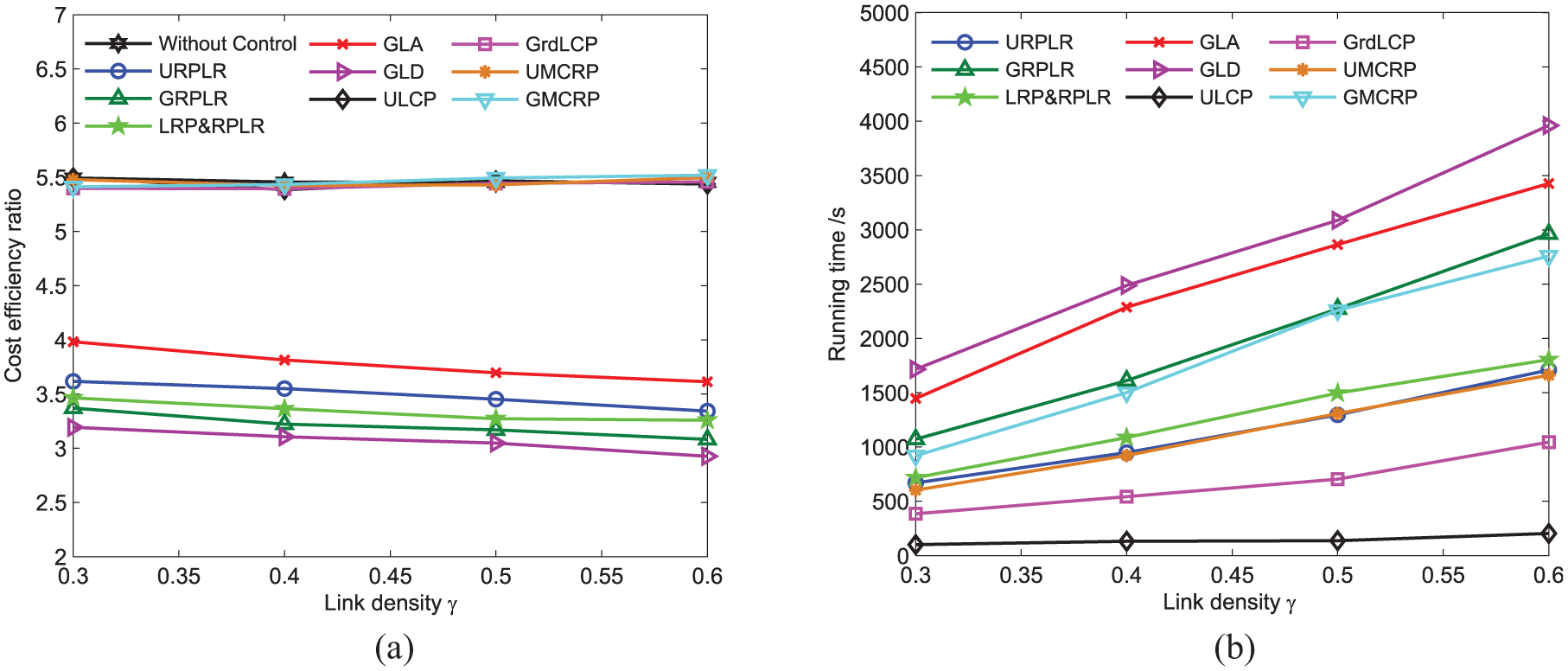
Simulation result in larger networks with different link densities (
Simulation for hybrid LEO/GEO satellite-based sensor networks
LEO satellite-based sensors are increasingly used in the Earth observations. The high-resolution measurements of these LEO satellite-based sensors generate substantial quantities of scientific data that must be transmitted to the ground station. However, due to the low orbit (400–900 km altitude), LEO satellite usually has small visibility windows (around 10 min) with ground stations. These small visibility windows reduce the communication chance between LEO satellite-based sensors and ground stations and result in a communication bottleneck. To address this problem, many space agencies have proposed the use of GEO satellites as stationary relay points, for example, the Transformational Satellite Communications System (TSAT)45,46 and NASA’s LEO/GEO satellite network proposal. 21 GEO satellites usually have long visibility windows with LEO satellites, and GEO satellites are always visible to the ground stations. Hence, the relay of GEO satellites can eliminate the communication bottleneck and provide a continuous, flexile, data-stream downlink for LEO satellite-based sensors. This new, more complex, spacecraft network topology is time-varying and predictable. It cannot be managed using traditional, manually commanded, point-to-point communication. The topology control of it is important.
As shown in Figure 10, in this simulation scenario, we consider a hybrid LEO/GEO satellite-based sensor network with three GEO satellites, six LEO satellite-based sensors, and three ground stations. Both LEO and GEO satellites are operated in Walker Constellation. 47 The detailed orbit parameters of each satellite are described in Table 1. We use 554 km as the altitude of LEO satellites because the recursive period 48 of orbits with this altitude is 1 day. Furthermore, LEO satellite-based sensors are usually in sun-synchronous orbit, 48 so the inclination of the orbit is 97.5°. The longitudes of three GEO satellites’ foot node are 110°E, 10°W, and 130°W, respectively. The locations of ground stations are shown in Table 2. The downward beam-width of each GEO satellite and LEO satellite is 18° and 129.9°, respectively.

Architecture of hybrid LEO/GEO satellite-based sensor network.
Parameters of satellite nodes.
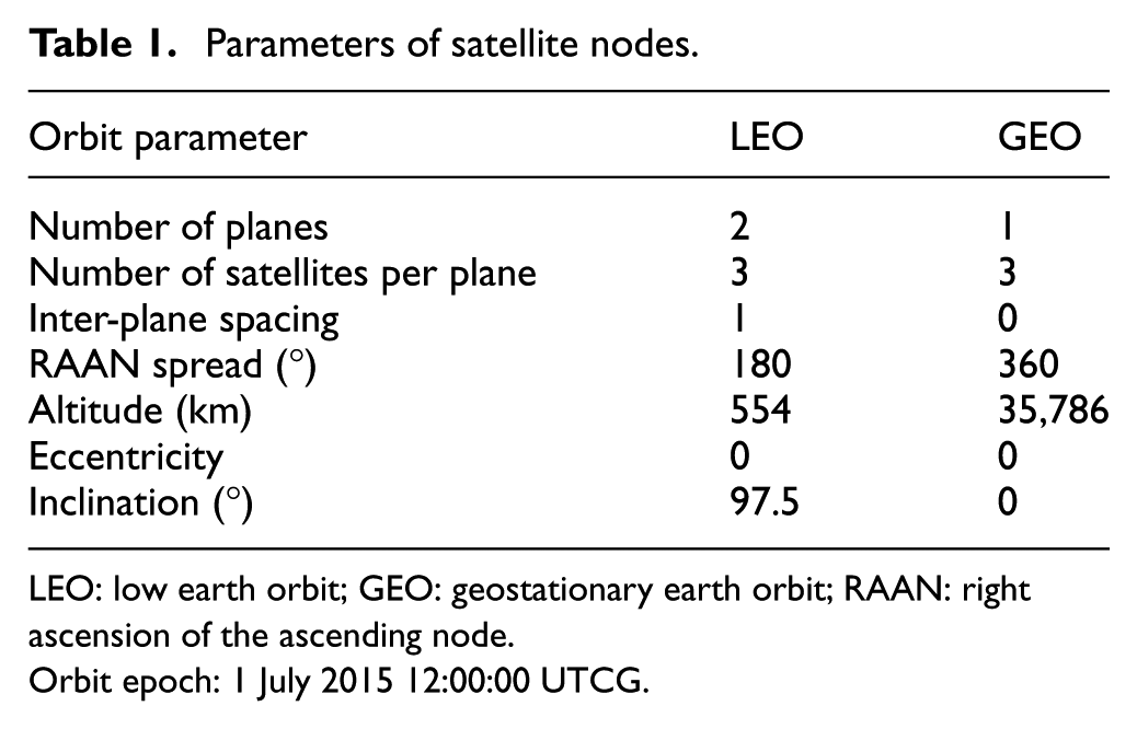
LEO: low earth orbit; GEO: geostationary earth orbit; RAAN: right ascension of the ascending node.
Orbit epoch: 1 July 2015 12:00:00 UTCG.
Ground station locations.

Therefore, possible links in this network are shown in Figure 11(a), which form the LEO/GEO network topology among all nodes. For clarity, not all possible links are shown here (e.g. inter-LEO and GEO satellite links). Since all ground stations are connected by Internet, we can use a virtual node to replace them (in STK, ground stations are combined into a constellation). Figure 11(b) shows the corresponding space–time graph model of Figure 11(a), where three ground stations are merged into one single virtual node. Notice that, unlike the connectivity from nodes to all other nodes in random networks, we only concern the connectivity from LEO satellites to the ground stations. Each link of space–time graph in this simulation is weighted as follows. For all spatial links: (1) link cost is proportional to the average distance of two vertices during one time slot; (2) link efficiency is randomly chosen from 1 to 10; and (3) link unreliability is randomly chosen from 0.01 to 0.05. For all temporal links, we assume that they have zero cost and perfect reliability, that is, both the cost efficiency ratio and unreliability are 0. Since the cost efficiency ratio of each temporal link is 0, we only compute the cost efficiency ratio of spatial links here.

Topology of hybrid LEO/GEO satellite-based sensor network: (a) the network topology with with time-varying links and (b) the corresponding space–time graph.
In this simulation, we use STK to calculate node parameters (e.g. position, etc.) and link parameters (e.g. range, duration, etc.). Then, node and link parameters generated from STK are exported to MATLAB for further processing and analysis. Figure 12 shows a snapshot from STK scenario. The start epoch and stop epoch of the STK scenario are 1 July 2015 12:00:00 UTCG and 2 July 2015 12:00:00 UTCG, respectively, that is, 24-hduration. We divide this 24 h into 144 topology management time equally, that is, there are 144 space–time graphs with

A snapshot of the STK scenario.
Figure 13 shows the simulation results over this LEO/GEO satellite network, the unreliability bound here is

Simulation results on the LEO/GEO satellite network
Conclusion
We studied the topology control problem in predictable time-varying spacecraft networks with unreliable links, using a space–time graph model weighted by cost, efficiency, and unreliability. Compared with most existing models, this model includes both temporal and spatial topology information. We first proved that this topology control problem is NP-hard, then we proposed five heuristic algorithms. Different from previous works, our algorithms not only consider the total cost of the network topology but also consider the cost efficiency ratio and unreliability. Simulation results from random space networks and hybrid LEO/GEO satellite-based sensor network demonstrated the efficiency of our proposed algorithms.
However, it is also seen that our algorithms still have some limitations: (1) we have assumed that only one-hop transmission is allowed during each time slot in this space–time graph model, which makes multi-hop to be transformed to virtual links; (2) we still assumed that the predictions of links and unreliability are feasible, hence the performance may degrade when unpredictable events happen. Therefore, in our future works, we will (1) design more efficient space–time graph model which allows multi-hop in one time slot; (2) design algorithms to adapt the unpredictable events rather than take them as unreliable probability.
Footnotes
Handling Editor: Kavita Pandey
Declaration of conflicting interests
The author(s) declared no potential conflicts of interest with respect to the research, authorship, and/or publication of this article.
Funding
The author(s) disclosed receipt of the following financial support for the research, authorship, and/or publication of this article: This work was supported by Innovative Foundation for Young Scholars of Space Engineering University under Grant No. 2019-017.