Sage Journals: Discover world-class research

Abstract

For the current situation of the large error in civil satellite positioning data resulting in the calculation of smaller mileage by the polyline method than the actual mileage, a new method of mileage statistics has been proposed in this article. First, the original trajectory data are preprocessed to eliminate data errors. Second, based on the principle of shape approximation, it is preferred to implement the quadratic B-spline curve to accurately fit the mileage trajectory curve, comparing various curve fitting methods. Then, based on the trajectory curve control point data, the mileage statistics formula is derived, and the accurate mileage statistics method for non-precision satellite positioning signals is realized. Finally, the road test is carried out by using the photoelectric non-contact five-wheel instrument and GPS equipment. The polyline method and curve fitting method are used to generate contrastive curve and calculate the mileage, respectively. Taking photoelectric five-wheel data as the accurate mileage, the error analysis is carried out. The results show that the deviation between calculated and actual mileage values is less than 1%. Therefore, this method can meet the user’s requirements for fleet management.

Keywords

Traffic engineering track mileage curve fitting GPS

Introduction

Mileage statistics is an important basis for vehicle maintenance, workload assessment, fuel consumption statistics, tire management, and fatigue driving warning in a fleet management. A normal mileage statistics method mainly includes the odometer measurement, the special instrument measurement, and the GPS measurement. Among them, the odometer data are easy to read, continuously available, and low cost. However, it also has the weakness of large error, poor real-time performance, and the possibility of data fraud due to its manual recording method. The special instrument measurement method usually adopts a photoelectric five-wheel system, and the measurement result is accurate and reliable. However, the cost of the equipment is high, and the installation and debugging are troublesome. It is only suitable for the experimental measurement of standard road sections but not suitable for fleet management. The mileage statistics based on GPS data is a low-cost method, which can automatically acquire data and is more accurate than the odometer method. So, it is considered to be the most popular way at present. However, due to the larger error of the original GPS data compared with the error by the special instrument, the data correction is required.^1,2

At present, the positioning accuracy of civil GPS is about 10 m. Real-time kinematic (RTK) or GPS-based inertial navigation system (INS) can improve the positioning accuracy to the centimeter level. However, high-precision positioning systems are costly and not suitable for civilian applications.^3,4 Zeng et al.⁵ and Patire et al.⁶ analyzed and studied the civil GPS signal error and the data fusion. Xie⁷ and Li et al.⁸ used the map matching method to process the GPS data and the broken-line method to calculate the mileage, and the error was between 3% and 5%. Most of the related research focuses on GPS trajectory data processing methods. In trajectory mileage statistics, they all use polygonal segments to generate trajectory line and then use the length accumulation method to calculate the mileage. Even so, all of them have not deduced the precise formula for calculating the mileage after trajectory fitting. Therefore, the current trajectory fitting and the mileage statistics methods are inadequate.^9,10 In order to guarantee the precision of trajectory mileage, the second-order B-spline curve formula is used to fit the trajectory line based on the preprocessing of the original trajectory data. Besides, the precise mileage calculation formula is deduced, which provides a reference for the research of GPS trajectory data.

Trajectory data preprocessing

Trajectory lines normally consist of a series of position points, which are organized chronologically to describe the spatiotemporal locus movement of an object. Define any track T_r as

T_{r} = p_{0} \to p_{1} \to \dots p_{i} \to p_{m - 1}

(1)

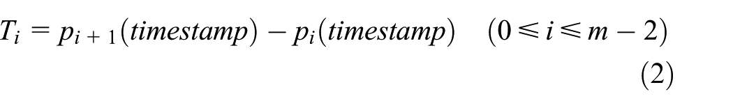
where p_i = (longtitude, lattitude, timestamp) is the data structure of each track point, and the variables are longitude, latitude, and positioning time, respectively. The m track points p₀ to p_m–₁ are distributed according to time series. The time interval of adjacent location points in the trajectory can be expressed as

T_{i} = p_{i + 1} (timestamp) - p_{i} (timestamp) (0 ⩽ i ⩽ m - 2)

(2)

The trajectory data errors mainly include the latitude and longitude errors caused by various factors, and the missing key points caused by $T_{i}$ are too large. Therefore, the original trajectory data need to be preprocessed, including static error point (zero point drift) processing, off-route singular point processing, and key missing data compensation during driving.^11,12

Static error point processing

Liu et al.¹³ and Gong et al.¹⁴ have done relevant research on GPS static drift point processing. Most of the literature uses the data filtering method for processing, which has a high probability of large error. In order to avoid large errors and simplify the calculation process, the gravity center method is adopted in this article.

Dift point identification

If the data obtained from GPS terminal equipment contain ACC (Accessory switch) which is a signal representing the engine switch, all GPS data which can indicate the engine shutdown state during a continuous time period can be regarded as zero drift data. If the engine switch signal is not obtained by GPS, the original GPS point data sequence needs to be judged. Zero drift point needs to satisfy two conditions, one is that the velocity is lower than the threshold in the continuous time period, and the other is that the direction information of each continuous coordinate point is inconsistent. That is to say, the data points satisfying the two conditions simultaneously in a certain period of time are identified as the zero drift data.

Drift point processing

1. Determine the coordinate values of discrete points in a new coordinate system.

GPS adopts the WGS84 coordinate system, which is not intuitive and complex in our calculation. Therefore, it is necessary to reset the coordinate origin and coordinate the original data in the new coordinate system. The coordinate value of the new coordinate origin in the WGS84 coordinate system is calculated according to the following equation

O_{x} = \frac{\sum_{i = 1}^{n} x_{i}}{n}, O_{y} = \frac{\sum_{i = 1}^{n} y_{i}}{n}

(3)

The new coordinate value of discrete points is calculated as follows

x_{i}' = x_{i} - O_{x}, y_{i}' = y_{i} - O_{y}

(4)

2. Construct a polygon and calculate the coordinates of the center of gravity.

Determine the quadrants of discrete points in the new coordinates and calculate the angle value, which is used as the sorting basis. After resorting, the data sequence is A_i(X_i, Y_i) (i = 1, 2,…N) and connect each data point in the order of the angle value to form a polygon. According to the polygon area theorem, the polygon center of gravity position can be calculated.

Given theorem 1: the area of the N-edge polygon with A_i(X_i, Y_i) (i = 1, 2…N) as the apex is (when the boundary A₁, A₂…A_n constitute a counterclockwise loop, take (+), and a clockwise loop takes (–))

S = \pm \frac{1}{2} \sum_{i = 1}^{n} [\begin{matrix} x_{i} & x_{i + 1} \\ y_{i} & y_{i + 1} \end{matrix}], Setting : x_{n + 1} = x_{1}, y_{n + 1} = y_{1}

(5)

The center of polygon gravity $G (\tilde{x}, \tilde{y})$ can be calculated from theorem 1

\begin{matrix} \tilde{x} = \frac{\sum_{i = 1}^{n} (x_{i} + x_{i + 1}) [\begin{matrix} x_{i} & x_{i + 1} \\ y_{i} & y_{i + 1} \end{matrix}]}{3 \sum_{i = 1}^{n} [\begin{matrix} x_{i} & x_{i + 1} \\ y_{i} & y_{i + 1} \end{matrix}]}, \\ \tilde{y} = \frac{\sum_{i = 1}^{n} (y_{i} + y_{i + 1}) [\begin{matrix} x_{i} & x_{i + 1} \\ y_{i} & y_{i + 1} \end{matrix}]}{3 \sum_{i = 1}^{n} [\begin{matrix} x_{i} & x_{i + 1} \\ y_{i} & y_{i + 1} \end{matrix}]} \end{matrix}

(6)

According to the abovementioned method, the center of gravity coordinates of all the static drift discrete points in the new coordinate system can be calculated.

3. Calculate the original coordinate value of the point $G (\tilde{x}, \tilde{y})$ , that is, the coordinate value in the WGS84 coordinate system

x_{0} = \tilde{x} + O_{x}, y_{0} = \tilde{y} + O_{y}

(7)

Combine the trajectory data

Delete all identified drift points in the data sequence T_r, as T_r₁. Taking the time value of the first point in the sequence of deleted drift points as the timestamp attribute value of G₀(x₀, y₀) point and then inserted into T_r₁. Reordering all points by timestamp attribute, and it is recorded as T_r₂.

Taking the zero drift point processing as an example, the test vehicle stays for 1 h and the drift data points have 22 points. The contrasting trajectory before and after processing is shown in Figure 1.

Figure 1.

Comparison of zero drift trajectory before and after processing.

Error point processing in motion

There are two types of singular points caused by unstable GPS signals during traveling, one is the large error points, and the other is the small error points deviating from the route. For large error points, the curvature elimination method or the three-point velocity threshold method is usually used for deletion. The curvature elimination method is more accurate in the case of highways or suburban roads with little curvature, but in urban roads, there is a risk of eliminating normal data when there is a right-angle or greater than right-angle turning.¹⁵ In this article, the track line contains urban sections; therefore, three-point velocity threshold method is adopted to process large error points based on continuous positioning points. The specific methods have been reviewed in the literature.¹⁶ For small deviation points, the geometric primitive method is usually used for identification first, and the detailed identification methods have been reviewed in the literature.^17,18 Then, the deviation points are modified, and the arc projection algorithm is used to project the deviation point to the current section.¹⁹ As shown in Figure 2, the deviation point is identified as M(x_M, y_M), and two adjacent data points without deviation are determined as A(x_A, y_A), B(x_B, y_B). Project point M on the line segment $\vec{AB}$ to obtain a new point M′ whose time attribute is the same as M and replace M by $M'$ .

Figure 2.

Deviation points projection diagram.

The calculation method of the M′ point coordinates is as follows.

1. Calculate the angle $θ$ between M and the road segment. When the coordinates of three points are known, the value $θ$ can be calculated by the formula of trigonometric function

\begin{matrix} ∠ θ = Arc \cos \\ {\frac{[(x_{A} - x_{B}) (x_{M} - x_{B}) + (y_{A} - y_{B}) (y_{M} - y_{B})]}{| AB ‖ BM |}} \end{matrix}

(8)

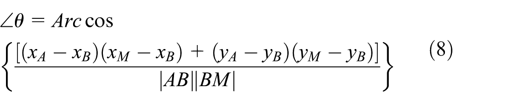
where $| AB | = \sqrt{{(y_{M} - y_{B})}^{2} + {(x_{M} - x_{B})}^{2}}, | BM | = \sqrt{{(y_{A} - y_{B})}^{2} + {(x_{A} - x_{B})}^{2}}$ .

2. Calculate the projection distance of BM section on the road: $L' = | L 1 \times \cos θ |$ , $L 1 = | BM |$ .

3. Calculate the projection coordinates of the offset point

\frac{A M'}{AB} = \frac{| AB | - L'}{| AB |} = \frac{x' - x_{A}}{x_{B} - x_{A}} = \frac{y' - y_{A}}{y_{B} - y_{A}}

(9)

Substitute $| AB |$ , $L'$ into formula (8) to calculate the coordinate value of $M' (x', y')$ .

Because of the occlusion and location interval of GPS signal, there is a lack of key data in the GPS data sequence, which has a great impact on the trajectory curve and the mileage. The key missing data can be compensated according to the method in the literature.^20,21

According to the abovementioned method, the track point data are processed. After the processing, the GPS data sequence is recombined. It is assumed that there are n + 1 track point data, the track sequence is denoted as

T_{r}' = p_{0} \to p_{1} \to \dots p_{i} \to p_{n}

(10)

Trajectory curve fitting

Curve fitting is to minimize variance between the actual data and prediction data using a suitable regression approach.^9,22 The methods of curve fitting mainly include Bessel curve, B-spline curve, parabolic adjustment curve, and cubic parameter spline curve. Parabolic and cubic spline curves require strict passing of feature points, which results from GPS positioning point errors, and so this method is not suitable for curve fitting of GPS positioning points. Bessel curve and B-spline curve methods do not pass all known points, the generated curve has the minimum sum of “distance” from all known points, and so they are suitable for curve fitting when there are errors in the known data points. Bessel curve passes through the starting point and end point, and its points have overall controllability. If some data point changes locally, the trajectory curve needs to be regenerated, and the calculation process is complicated. The B-spline curve is a kind of curve developed on the basis of the Bezier curve. It overcomes the inconvenience caused by the overall controllability of the Bezier curve, and the most commonly used are the quadratic and cubic B-spline curves. In terms of curve continuity, cubic is better than quadratic, cubic can achieve second derivative continuity, and in terms of the approximation of the generated polygon curve, the quadratic is better than cubic.^23–25

In this part, according to the shape approximation, the trajectory curve is fitted by the quadratic B-spline method, which is designed for three discrete points, and the piecewise fitting method can be adopted for multiple GPS data points. Compared with the Bezier curve, a curve segment of piecewise quadratic B-spline is only related to the corresponding two broken line segments and three control polygon vertices. Changing one of the vertices only affects the three spline curve segments. Therefore, when the original positioning point may change, this method can reduce the computational complexity and increase the computing speed. However, the B-spline curve does not pass through the start and end points; therefore, the boundary processing is required in the curve fitting.

The elements in the trajectory are $P_{i} (i = 0, 1, 2 \dots n)$ . The quadratic B-spline curve is used to generate a trajectory curve after piecewise fitting of the data points. Follow the following steps.

Boundary processing

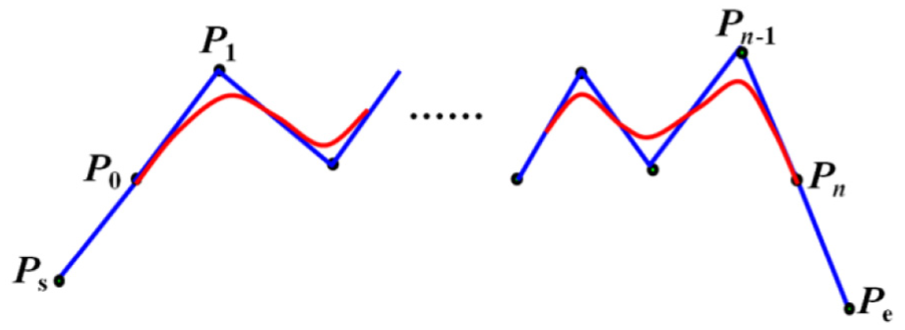
The B-spline curve has the following characteristics: the starting point is the midpoint of $P_{0}, P_{1}$ , and it is tangent to $P_{0}, P_{1}$ . The ending point is the midpoint of $P_{n - 1}, P_{n}$ , and it is tangent to $P_{n - 1}, P_{n}$ . It can be seen from this feature that the trajectory generated by the B-spline curve does not pass through the positioning starting and ending points, and so the boundary processing of the original data points is required. As shown in Figure 3, add two points $P_{s}, P_{e}$ , $P_{s}$ on the extension line of $P_{1} P_{0}$ , and $P_{1} P_{0} = P_{0} P_{s}$ , $P_{e}$ on the extension line of $P_{n - 1}, P_{n}$ , and $P_{n - 1} P_{n} = P_{n} P_{e}$ . In the data sequence $P_{i}$ , the $P_{0}$ coordinate value is replaced by $P_{s}$ , and the $P_{n}$ is replaced by $P_{e}$ . That is, after the boundary processing is completed, the new data sequence is $P_{i} (i = 0, 1, 2 \dots n)$ , where $P_{0} = P_{s}$ , $P_{n} = P_{e}$ , and the coordinate values of the other points remain unchanged.

Figure 3.

The boundary processing schematic.

Realization of curve generation

Taking $P_{0} (x_{0}, y_{0}), P_{1} (x_{1}, y_{1}), P_{2} (x_{2}, y_{2})$ as control points to draw first curves as an example, the generation method of the B-spline curve is explained. The parametric component equation can be calculated by quadratic B-spline curve formula as follows

{\begin{matrix} x (t) = \frac{1}{2} (x_{0} + x_{1}) + (x_{1} - x_{0}) t + \frac{1}{2} (x_{0} - 2 x_{1} + x_{2}) t^{2} \\ y (t) = \frac{1}{2} (y_{0} + y_{1}) + (y_{1} - y_{0}) t + \frac{1}{2} (y_{0} - 2 y_{1} + y_{2}) t^{2} \end{matrix} (t \in [0, 1])

(11)

Set the smoothness coefficient k, and segment the parameter t with the step length: $t = 1 / k$ . The larger the k, the more smooth the generated curve will be, but the amount of computation is larger. Taking $k = 100$ , the step length is 0.01, $t = {0, 0.01, 0.02, 0.03, \dots 1}$ , a total of 101 data, and then calculate the coordinate values corresponding to different t values and connect the coordinate points to get the first B-spline curve. The same method is used to draw the second curve at the control point of $P_{1}, P_{2}, P_{3}$ and then generate the $(n - 1) th$ curve at the control point of $P_{n - 2}, P_{n - 1}, P_{n}$ . With this approach, a total of n segmentation curves are generated. Each curve has the same tangent line at each connection point, thus the quadratic B-spline curve has a $C^{1}$ -level continuity which satisfies the smoothing requirements of trajectory curve.

Trajectory mileage calculation

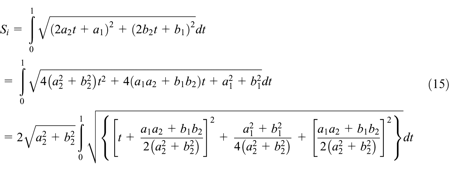
The quadratic B-spline curve is continuous and derivable on the parameter interval [0,1]. According to the arc length formula of parametric equation, it can be known that the arc length of the ith segment can be calculated by the following formula

S_{i} = \int_{0}^{1} \sqrt{x' {(t)}^{2} + y' {(t)}^{2}} dt

(12)

Write formula (11) as the standard form of the quadratic B-spline parameter component equation

{\begin{matrix} x (t) = a_{0} + a_{1} t + a_{2} t^{2} \\ y (t) = b_{0} + b_{1} t + b_{2} t^{2} \end{matrix} (t \in [0, 1])

(13)

Deriving the parameter components in equation (13)

{\begin{matrix} x' (t) = 2 a_{2} t + a_{1} \\ y' (t) = 2 b_{2} t + b_{1} \end{matrix} (t \in [0, 1])

(14)

Substitute formula (12)

\begin{matrix} S_{i} = \int_{0}^{1} \sqrt{{(2 a_{2} t + a_{1})}^{2} + {(2 b_{2} t + b_{1})}^{2}} dt \\ = \int_{0}^{1} \sqrt{4 (a_{2}^{2} + b_{2}^{2}) t^{2} + 4 (a_{1} a_{2} + b_{1} b_{2}) t + a_{1}^{2} + b_{1}^{2}} dt \\ = 2 \sqrt{a_{2}^{2} + b_{2}^{2}} \int_{0}^{1} \sqrt{{{[t + \frac{a_{1} a_{2} + b_{1} b_{2}}{2 (a_{2}^{2} + b_{2}^{2})}]}^{2} + \frac{a_{1}^{2} + b_{1}^{2}}{4 (a_{2}^{2} + b_{2}^{2})} + {[\frac{a_{1} a_{2} + b_{1} b_{2}}{2 (a_{2}^{2} + b_{2}^{2})}]}^{2}}} dt \end{matrix}

(15)

Let $m = t + (a_{1} a_{2} + b_{1} b_{2} / 2 (a_{2}^{2} + b_{2}^{2})), c = a_{1}^{2} + b_{1}^{2} / 2 (a_{2}^{2} + b_{2}^{2}) - [a_{1} a_{2} + b_{1} b_{2} / 2 (a_{2}^{2} + b_{2}^{2})]^{2}$

When $t = 0$ , $m = a_{1} a_{2} + b_{1} b_{2} / 2 (a_{2}^{2} + b_{2}^{2})$ . When $t = 1$ , $m = 1 + a_{1} a_{2} + b_{1} b_{2} / 2 (a_{2}^{2} + b_{2}^{2})$

Substitute $m, c$ and integral range into formula (15), and according to the definite integral formula, the calculation is as follows

\begin{matrix} S_{i} = 2 \sqrt{a_{2}^{2} + b_{2}^{2}} \int_{\frac{a_{1} a_{2} + b_{1} b_{2}}{2 (a_{2}^{2} + b_{2}^{2})}}^{1 + \frac{a_{1} a_{2} + b_{1} b_{2}}{2 (a_{2}^{2} + b_{2}^{2})}} \sqrt{m^{2} + c} dm \\ = 2 \sqrt{a_{2}^{2} + b_{2}^{2}} \\ [\frac{m}{2} \sqrt{m^{2} + c} + \frac{c^{2}}{2} \ln (m + \sqrt{m^{2} + c})] |_{\frac{a_{1} a_{2} + b_{1} b_{2}}{2 (a_{2}^{2} + b_{2}^{2})}}^{\frac{a_{1} a_{2} + b_{1} b_{2}}{2 (a_{2}^{2} + b_{2}^{2})}} \end{matrix}

(16)

Suppose that the three control points of the ith curve are ${(x_{0}, y_{0}), (x_{1}, y_{1}), (x_{2}, y_{2})}$ , the parameters in the above equation can be rewritten by

{\begin{matrix} a_{0} = x_{0} \\ a_{1} = 2 (x_{1} - x_{0}) \\ a_{2} = x_{0} - 2 x_{1} + x_{2} \end{matrix} {\begin{matrix} b_{0} = y_{0} \\ b_{1} = 2 (y_{1} - y_{0}) \\ b_{2} = y_{0} - 2 y_{1} + y_{2} \end{matrix}

Substituting $a_{1}, a_{2}, b_{1}, b_{2}$ into formula (14), the arc length of the piecewise curve can be obtained

Mile = \sum_{i = 1}^{n - 1} S_{i}

(17)

Experiment and result analysis

Test environment

The test vehicle is equipped with both a photoelectric non-contact five-wheel instrument and a GPS device, the GPS device uploads positioning data to the server through GPRS network, and users can obtain trajectory data through computer client, as shown in Figure 4. The photoelectric five-wheel instrument has a high precision used to measure speed and distance, which has an accuracy of ±0.5%, and the average value of five measurements on the same route is used as the standard mileage in the whole experiment. The A300 civil non-high-precision GPS device of Beijing Ding Technology Co, Ltd was selected in this experiment, the positioning interval is set as 30 s, the stall dormancy positioning interval is 120 s, and the heartbeat interval is 60 s. A road in Qingdao including urban roads and suburban expressway was chosen as the test route without tunnel culvert. The route is set as departure at point A (Start), getting to destination B (End), and then going back to point A. The stay times are as follows: 2 h before departure at A, 1 h on return at A, 2 h at B, and unlimited travel time. Five tests were conducted on the same route.

Figure 4.

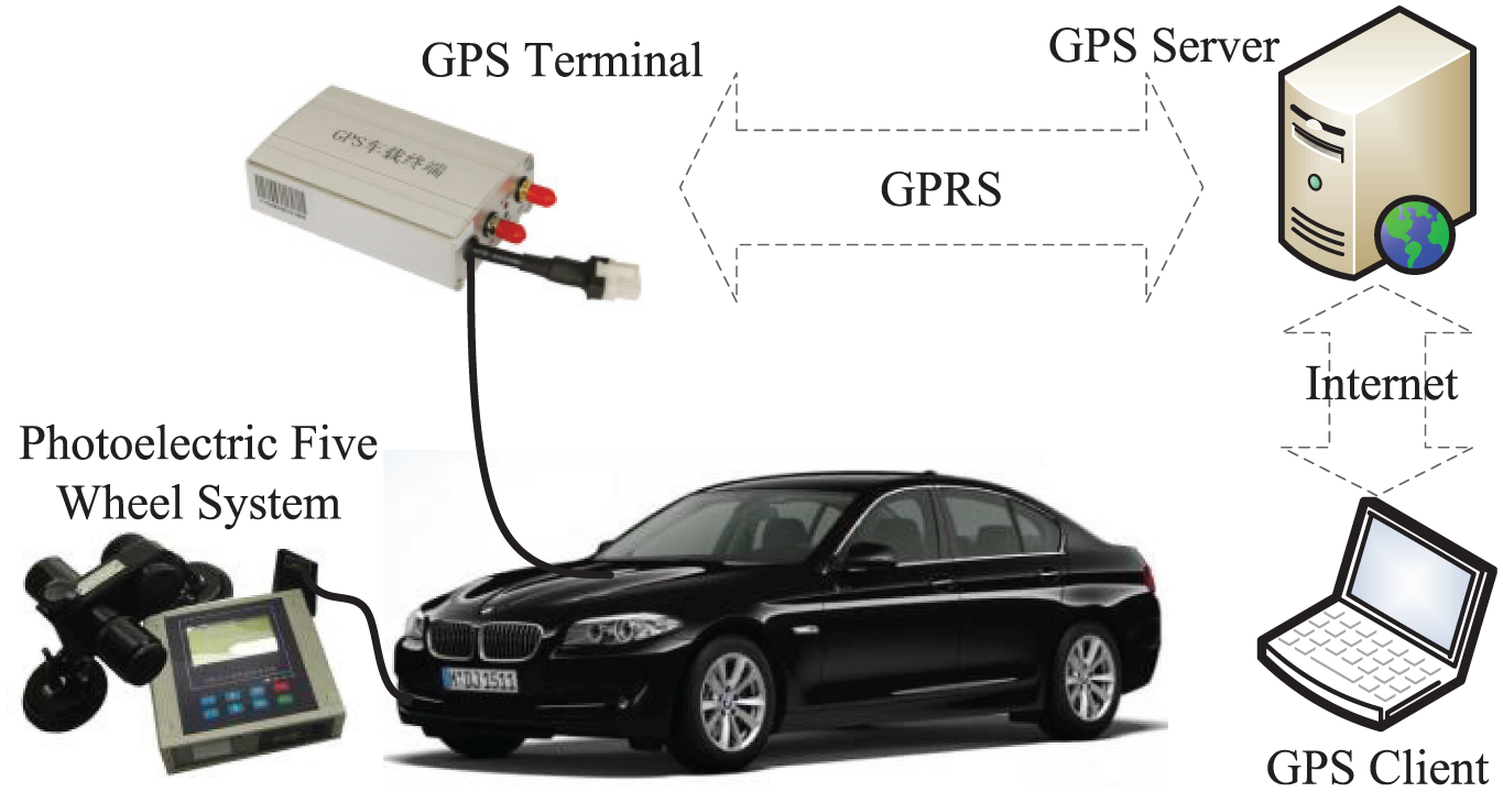
Diagram of test system.

Test result

A total of 1650 data were obtained from the five measurements, and each data includes the information of longitude, latitude, speed, altitude, and positioning time. The preprocessed results of one set of go and return measurements with 326 points are as follows: identify drift position point 2 and eliminate 178 drift data, identify 0 point with large error, identify and process a total of 46 small deviation points, and compensate 36 missing points. After processing, the data sequence is regenerated, totaling 163 points of data.

The broken line method is used to connect the trajectory points directly in time sequence, and the trajectory generated by this method is shown in Figure 5. The going trip is marked as red, and the return is blue. The total length (round trip) of all broken line segments is 40.99 km.

Figure 5.

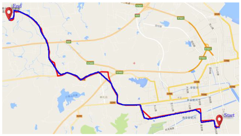
The trajectory line curve based on original data.

The trajectory curve generated using the secondary B-spline curve algorithm is shown in Figure 6. The new mileage statistics formula is used to calculate the mileage (including the going and return), and the result is 43.34 km.

Figure 6.

The fitting trajectory curve based on processed data.

Result analysis

Curve fitting effect

In Figure 5, the trajectory is in the form of broken line segment. Due to the large interval between positioning points, the trajectory line is not smooth and poorly visible. Due to positioning error and GPS data loss, there is no overlap between the going and return curves, especially on the road sections with more turns. In Figure 6, the going and return trajectory lines go through the same route and basically coincide. The curve is smooth with better effect. The zero drift data points at the stop point have been reasonably processed. Error points and singular points data have been processed. The missing data at the intersection have been compensated. After comparing the two sets of curves, it is known that the fitting curve is closer to the original trajectory.

Mileage error analysis

The average value of five measurements by photoelectric five-wheel is 43.08 km. Taking these data as the accurate mileage, the measurement results are shown in Table 1.

Table 1.

Error analysis for mileage statistics.

Id	Odometer method (km)	Polyline method (km)	Fitting method (km)	Relative error of odometer method (%)	Relative error of polyline method (%)	Relative error of fitting method (%)
1	40.2	40.99	43.34	−6.69	−4.85	0.60
2	40.7	41.52	42.81	−5.52	−3.62	−0.63
3	39.9	41.62	43.15	−7.40	−3.39	0.16
4	40.5	42.03	42.73	−5.99	−2.44	−0.81
5	40.9	41.98	43.02	−5.06	−2.55	−0.14

From Table 1, we can see that the deviations for the relative odometer method all exceed 5%, and so it is not suitable for accurate mileage statistics. The relative error range of the polyline method is −2.44% to −4.85%, which has a large fluctuation range. This method ignores the curvature of the vehicle’s route and replaces the curve with a straight line. So, the mileage value is always lesser than normal, which can satisfy the general monitor system requirements, but not for monitoring systems with higher accuracy requirements. The fitting method uses quadratic B-spline curve algorithm to fit the trajectory, whose effect is close to the original trajectory, and the curve segment cumulative integral algorithm is used to calculate the mileage. In the five experimental results, taking the average value of five-wheel system result as the standard mileage, the average error of odometer method, polyline method, and fitting method are −6.13%, −3.37%, and 0.16%, respectively. It can be seen that the accuracy of the fitting method is 5.97% higher than the odometer method and 3.12% higher than method, which satisfies the requirement of accurate mileage statistics.

Conclusion

In this article, the non-high-frequency civil satellite data are preprocessed, the trajectory curve is fitted, and the accurate mileage statistical formula is derived. We conclude that;

Aiming at various errors existing in the original GPS data, the original trajectory data were preprocessed: a gravity center method is proposed for the zero drift data, the projection method is used to process the trajectory deviation point, and the key missing data are compensated.

Aiming at the problems existing in the traditional polyline trajectory method, the trajectory curve fitting method based on the quadratic B-spline curve is presented, and the calculation formula of the trajectory mileage is derived. Based on this, the accurate mileage statistics of the non-precision satellite positioning signal are realized, and the mileage statistics in the fleet management is further improved.

According to the new method, an experimental test was carried out, and the relative errors of odometer method, polyline method, and fitting method were compared and analyzed. The analysis results show that the error of the quadratic B-spline fitting method mileage is within 1%, and the average error is reduced by 5.97% compared with the odometer method, and by 3.12% compared with the polyline method, which meets the application requirements for fleet management.

Footnotes

Handling Editor: Daming Zhou

Declaration of conflicting interests

The author(s) declared no potential conflicts of interest with respect to the research, authorship, and/or publication of this article.

Funding

The author(s) disclosed receipt of the following financial support for the research, authorship, and/or publication of this article: This study was supported by the Natural Science Foundation of China (grant nos: 61671262, 61871447, and 51806114).

ORCID iD

Chuijie Yi

References

Reddy

BNK

Naraimhulu

Prasad

SVS

et al . An efficient online mileage indicator by using sensors for new generation automobiles. In: International conference on advanced computing, networking and security, Mangalore, India, 15–17 December 2013, pp.199–203. New York: IEEE.

Sood

Willis

Jaekel

et al . Analyzing accuracy of GPS data for vehicular parameters. In: International conference on connected vehicles and expo, Shenzhen, China, 19–23 October 2015, pp.344–345. New York: IEEE.

Malleswaran

Vaidehi

Manjula

et al . Performance comparison of HONNs and FFNNs in GPS and INS integration for vehicular navigation. In: International conference on recent trends in information technology, Chennai, India, 3–5 June 2011, pp.223–228. New York: IEEE.

Adusumilli

Bhatt

Wang

A low-cost field re-configurable real-time GPS/INS integrated system-design and implementation. Exp Syst Appl 2013; 6: 112–115.

Zeng

Chen

Wang

L-J

et al . Multiple GPS data fusion algorithm based on principal curves and adaptive radius method. J China Rail Soc 2015; 37(2): 46–51.

Patire

Wright

Prodhomme

et al . How much GPS data do we need? Transp Res Part C: Emerg Technol 2015; 58: 325–342.

Xie

YD.

Research on GPS algorithm based on outliers filter for vehicle mileage. Harbin, China: Harbin Engineering University, 2017.

et al . Accurate localization based on GPS and image fusion for intelligent vehicles. J Transp Syst Eng Inform Technol 2017; 17(3): 112–119.

Zhou

Al-Durra

Matraji

et al . Online energy management strategy of fuel cell hybrid electric vehicles: a fractional-order extremum seeking method. IEEE T Ind Electron 2018; 65(8): 6787–6799.

10.

Zhou

Nguyen

Breaz

et al . Global parameters sensitivity analysis and development of a two-dimensional real-time model of proton-exchange-membrane fuel cells. Energ Convers Manage 2018; 162: 276–292.

11.

Moore

Watson

King

et al . Empirical modelling of site-specific errors in continuous GPS data. J Geodesy 2014; 88(9): 887–900.

12.

Azarbad

Mosavi

MR.

A new method to mitigate multipath error in single-frequency GPS receiver with wavelet transform. GPS Solut 2014; 18(2): 189–198.

13.

Liu

Huang

et al . GPS trajectory data drift processing method based on time series considering velocity constraints. J Geomat 2017; 42(1): 14–18.

14.

Gong

Sato

Yamamoto

et al . Identification of activity stop locations in GPS trajectories by density-based clustering method combined with support vector machines. J Mod Transp 2015; 23(3): 202–213.

15.

Zhang

Research on mobile positioning optimization technology based on multi-source information fusion. Beijing, China: Beijing University of Posts and Telecommunications, 2013.

16.

Fang

Tang

et al . GPS dynamic filter algorithm based on lifting wavelet transformation. J Transp Syst Eng Inform Technol 2013; 13(1): 43–48.

17.

Jiménez

Monzón

Naranjo

JE.

Definition of an enhanced map-matching algorithm for urban environments with poor GNSS signal quality. Sensors 2016; 16(2): 193.

18.

Schuessler

Axhausen

KW.

Processing raw data from global positioning systems without additional information. Transp Res Rec J Transp Res Board 2009; 2105: 28–36.

19.

Zhu

Cui

Liu

Method of map matching based on GPS terminal. Comp Sci 2013; 40(5): 291–295.

20.

Cai

WF.

Research on integrated navigation data fusion methods during GPS signal outages. Kirkland, WA: Northwest University, 2015.

21.

Zheng

Chen

New algorithm of GPS positioning in incomplete condition of temporal insufficient signal. J Univ Electron Sci Technol China 2009; 38(4): 496–500.

22.

Zhou

Al-Durra

Zhang

et al . Online remaining useful lifetime prediction of proton exchange membrane fuel cells using a novel robust methodology. J Power Sour 2018; 399: 314–328.

23.

Liu

Lin

. Research on the dynamometer diagram acquisition of rod pumping unit and curve fitting method. Manuf Autom 2014(11): 148–150.

24.

Albrecht

Beccari

Canonne

et al . Planar pythagorean-hodograph B-spline curves. Comp Aid Geomet Des 2017; 57(10): 57–77.

25.

Iglesias

Gálvez

Collantes

Multilayer embedded bat algorithm for B-spline curve reconstruction. Integr Comput Aid Eng 2017; 24(4): 1–15.

Research on the high-accuracy mileage statistics method based on the civil satellite data

Abstract

Keywords

Introduction

Trajectory data preprocessing

Static error point processing

Dift point identification

Drift point processing

Combine the trajectory data

Error point processing in motion

Trajectory curve fitting

Boundary processing

Realization of curve generation

Trajectory mileage calculation

Experiment and result analysis

Test environment

Test result

Result analysis

Curve fitting effect

Mileage error analysis

Conclusion

Footnotes

Declaration of conflicting interests

Funding

ORCID iD

References