Improved global stability condition analysis for time-delay fast active queue management scalable transmission control protocol

Abstract

The nonlinear time-delay fast active queue management scalable transmission control protocol model was studied in this article. By analyzing the boundedness properties for solution trajectory of the fast active queue management scalable transmission control protocol model, the iterative relations of fast active queue management scalable transmission control protocol trajectory bounds were obtained. Furthermore, we calculated the maximum growth direction of the delay term in the integral interval and applied the backward method to calculate the lower conservative bound corresponding to each time of the delay term. Therefore, the global stability parameter condition of fast active queue management scalable transmission control protocol, which was less conservative than the existing global stability conditions, was obtained in this article. The validity of the stability conditions obtained in this article was verified by NS-2 simulation experiment.

Introduction

Fast active queue management scalable transmission control protocol (FAST TCP) is a new TCP congestion control algorithm for large bandwidth-delay product networks.^1,2 The extensive experiments of FAST TCP had been conducted, and the results were promising.^3,4 However, intensive studies on the global stability of FAST TCP have not been carried out thus far, which remains as an open challenge. The stability of FAST TCP system was related to FAST TCP parameters and network parameters.^1–3 FAST TCP parameters include the number of protocol parameters $\alpha$ that was expected to remain as the data packets in the link buffer, gain parameter $\gamma$ of control law, and window update period $T$ . Network parameters include propagation delay $d$ and link bandwidth $c$ . When these two sets of parameters do not match, the stability of the system will be affected, so it was necessary to establish the relationship between these two sets of parameters to guide the selection of protocol parameters and to find an effective way to solve the public problem.^4,5

In Agrawal and Sherwood ⁵ and Cui and Andrew, ⁶ a guidance scheme of selecting protocol parameters using static mapping table according to link bandwidth was proposed. Agrawal and Sherwood ⁵ pointed out on the basis of experimental simulation that in a single-link network, the protocol parameter $\alpha$ should be greater than 0.0075 times the link bandwidth. However, the above two schemes did not consider another network parameter propagation delay, which was an empirical value strategy, and it was difficult to ensure the stability of the system under different network environments. In Chenmin ⁷ and Zhang et al., ⁸ pointed out that the FAST TCP protocol lacked global state and the control parameters were not easy to set, and an improved scheme based on measurement was proposed. The basic idea was to use measuring facilities distributed in the network to periodically monitor the network backbone. According to the measurement results, the protocol parameters were set by fuzzy control technique, and the bottleneck queue tended to a fixed length without relying on the router.

JT Wang et al. established the approximate continuous model of FAST TCP network congestion control in Wang et al. ³ and Zhang et al. ⁸ Based on the optimization theoretical framework, the nonlinear programming optimization model and the corresponding dual model for FAST TCP were established in Wei et al., ¹ Tan et al., ⁹ and Tang et al. ¹⁰ The Karush–Kuhn–Tucker condition theorem was adopted in Jacobsson et al. ¹¹ to prove that the above mentioned FAST TCP network congestion control model had a unique reachable equilibrium point. It was proved that this equilibrium point was the optimal solution of the above optimization model and the corresponding dual model. Wang et al. ³ proved that when round-trip delay was ignored and $\gamma \in (0,1]$ , the FAST TCP network congestion control can converge to the equilibrium point. A Tang et al. established an integral link model considering both TCP self-synchronization and dynamic characteristics of link end in Tan et al., ⁹ Tang et al., ¹⁰ and Jacobsson et al., ¹¹ and the Nyquist stability criterion was applied to prove that the FAST TCP system was locally stable on a single link when $\alpha >0$ , $\gamma \in (0,0.94)$ . K Jacobsson et al. ¹¹ improved the conclusions of Tan et al. ⁹ It was proved that the FAST system in multi-heterogeneous source and single-link networks was stable when the round-trip delay was bounded and the protocol parameters were $\alpha >1$ and $\gamma \in (0,0.93]$ . In Chen et al., ¹² Jacobsson, ¹³ and Nagaraj et al., ¹⁴ Kyungmo Koo et al. considered the more general case of taking different fixed values for the window update period, and the Lyapunov–Razumikhin theorem was applied to prove that the single-source single-link FAST TCP system was asymptotically stable when $\alpha >\mathrm{cd}$ or $\gamma d/T\in (0,1)$ . However, the FAST TCP model for stability analysis ignored the dynamic characteristics of the exponential smoothing filter and the queueing delay. Chen et al. ¹⁵ and Prasad et al. ¹⁶ established the continuous model of single-link single-connection FAST TCP network congestion control assuming that the window update period $T$ was an round-trip time (RTT) and proved that the FAST TCP system was asymptotic stability. The stability condition linked the two sets of parameters and can decouple the protocol parameters from other related parameters to guide the selection of protocol parameters. However, its FAST TCP model for stability analysis only considered the special case where the window update period $T$ was an RTT and ignored the exponential smoothing filter that was used to estimate the congestion feedback signal. So, there were some defects of conservative guidance scope and limited application scope. In summary, according to the stability conclusion of literature,^8–14 the following guidance scheme can be given.

In the case that the parameter $T$ was a RTT and $\gamma \in (0,0.93]$ and $d$ was bounded, the protocol parameters can be selected within the range of guidance $[1,\infty )$ to ensure the stability of FAST TCP system. This guidance scheme relaxed the selection range of protocol parameters but constrained other parameters. When other parameters did not meet the constraint conditions, the guidance scheme will be invalid, so the application range of the guidance scheme was limited.

According to the stability conclusion of literature,^15–18 the following guidance scheme can be given: select $\alpha >\mathrm{cd}$ under constrained conditions $\gamma d/T\in (0,1)$ or select $\alpha >0$ . Again, the scheme had the shortcoming of limited scope of application. If you selected the first condition $\alpha >\mathrm{cd}$ , it can guarantee the stability of the FAST TCP system. However, if the value was too large, it will increase the link queue delay, reduce the link utilization, and even cause the overflow of the link buffer queue and result in a large number of data packet losses, so that the network will appear as a violent oscillation phenomenon. If the second condition $\alpha >0$ was adopted, a smaller value can be selected, but other related parameters were constrained and the requirements $\gamma d/T\in (0,1)$ were satisfied.

The global stability of FAST TCP was studied for the case of single-link single-source network with maximal feedback delay instead of time-varying feedback delay in Prasad et al., ¹⁶ Koo et al., ¹⁷ and Choi et al. ¹⁸ The global stability condition was obtained using the Lyapunov–Razumikhin theorem, but the “constant” feedback delay had been incorrectly replaced with the time-varying feedback delay in the proof of the main theorem. ¹⁶ Koo et al. ¹⁷ corrected this crucial mathematical error and proposed an improved parameter condition for the global stability of FAST TCP with the time-varying feedback delay using a new analysis based on the Lyapunov–Razumikhin theorem and the linear matrix inequality (LMI) method. ¹⁷

In this article, an improved global stability condition of FAST TCP in a single-link single-source network was derived by analyzing the trajectory bounds of the FAST TCP model. ¹⁸ This condition provides a larger stability region of parameters as compared to the existing conditions described in Prasad et al., ¹⁶ Koo et al., ¹⁷ and Choi et al. ¹⁸

FAST TCP model

Network topology

At present, the network topology structure of network congestion control reported and studied in literature can be summarized as the three network topologies shown in Figures 1–3.

Figure 1.

Multisource multilink network topology.

Figure 2.

Multisource single-link dumbbell network topology.

Figure 3.

Single-source single-multilink network topology.

In this article, as in Tan et al. ⁹ and Koo et al., ¹⁷ the single-source single-multilink network topology shown in Figure 3 and the same nonlinear time-delay FAST TCP congestion control system were adopted. The research was carried out on the basis of Zhang et al., ⁸ Tan et al., ⁹ and Tang et al. ¹⁰ The design idea of FAST TCP was to use queue delay information at the source end to calculate the number of packets in the link buffer of FAST TCP connection, according to the actual number of packets left in the link buffer and the distance from the equilibrium point position, and adjust the sending window size to actively control the length of the buffer queue left in the link, so as to actively avoid buffer queue overflow and congestion. Although each FAST TCP connection works independently and does not communicate with each other, each connection can affect the queue length of the link end by controlling the number of packets left in the link end buffer, thus indirectly affecting the window adjustment strategy of other connections and realizing the distributed algorithm. Since each FAST TCP connection works independently and there was no direct communication between each connection, the global stability condition of this article can guide each FAST TCP connection to set protocol parameters to ensure the stable operation of each connection. Therefore, the research results of this article can be extended to the dumbbell network topology shown in Figure 2. Similarly, based on the research in this article, further research can be carried out under the network topology shown in Figure 3.

Network model

As shown in Figure 3, the topology of single-source single-link network was considered. FAST TCP protocol was adopted at the source end, buffer at the link end was large enough, and queue management algorithm of tail loss was adopted.

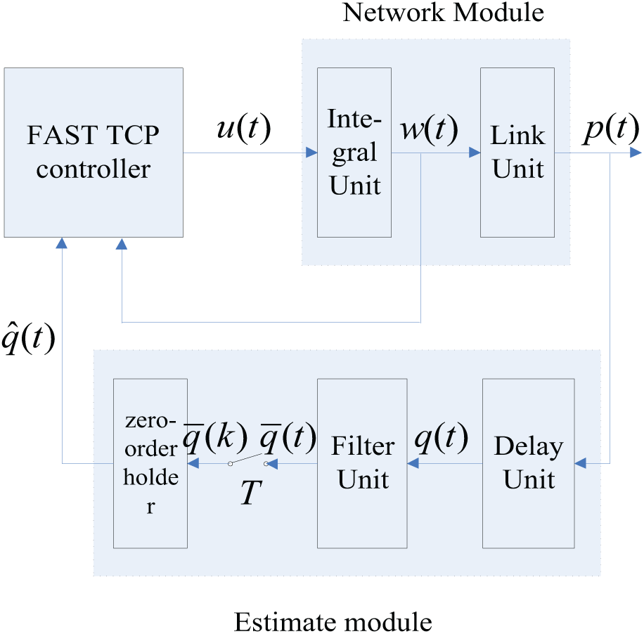
As shown in Figure 4, the congestion control model of FAST TCP network was mainly composed of network object module, estimation module, and FAST controller.

Figure 4.

FAST TCP network congestion control model.

The network object module was described as follows:

Integral unit: $\stackrel{·}{w}(t)=u(t)$ .

Link unit: $\stackrel{·}{p}(t)=\frac{1}{c}(\frac{w(t-R_f(t))}{d+p(t-R(t))}-c)$

The estimation model was described as follows:

Delay unit: $q(t)=p(t-R_b(t))$

Filter unit^9,10: $\stackrel{·}{\overline{q}}(t)=-\frac{3}{R(t)}\overline{q}(t)+\frac{3}{R(t)}\hat{q}(t)$

Zero-order holder: $\hat{q}(t)=\overline{q}(\mathrm{kT}),\forall t\in [\mathrm{kT},(k+1)T)$ , $k=1,2,...$

FAST TCP controller: $u(t)=\frac{\gamma }{T}(\alpha -\frac{w(t)}{d+\hat{q}(t)}\hat{q}(t))$

where $w(t)$ denotes source congestion window size at time $t$ , (packets); $u(t)$ denotes control signal at time $t$ ; $p(t)$ and $q(t)$ denote queuing delay of link end packet at time $t$ ; $R_f(t)$ denotes feedforward delay experienced from source to link (s); $R_b(t)$ denotes feedback delay from link to source (s); $R(t)$ denotes the RTT at time $t$ , assumed as $R(t)=R_f(t)+R_b(t)$ ; $d$ denotes the constant propagation delay, and $d=minR(t)$ , $R(t)=d+q(t)$ ; $q(t)=p(t-R_b(t))$ ; $\overline{q}(t)$ denotes the queue delay output by filtering link (s); $\hat{q}(t)$ denotes the queue delay output through the zero-order holder (s); $w(t-R(t))$ denotes source congestion window size at time $t-R(t)$ ; $c$ denotes the link capacity; $T$ denotes the window update period; $\gamma$ denotes the tuning parameter that determines the step size; and $\alpha$ is a positive protocol parameter that determines the total number of backlogs in link.

As described above, the following nonlinear time-varying delay FAST TCP model was derived with the single-link single-source network topology

$$\stackrel{·}{w}(t)=\frac{\gamma }{T}(\alpha -\frac{w(t)}{d+q(t)}q(t))$$

(1)

$$\frac{w(t-R(t))}{d+q(t)}=c$$

(2)

Assume that the network was under congestion, that is, $q(t)>0$ and $w(t)>\mathrm{cd}$ . ³

Substituting equation (2) into (1), we obtain the whole closed-loop delay system under congestion

$$\begin{array}{c}\stackrel{·}{w}(t)=f(w(t),w(t-R(t)))=r(\alpha -w(t)(1-\frac{\mathrm{cd}}{w(t-R(t))}))\hfill \\ w(t)={\varphi }_0>\mathrm{cd},t\in (-max(R(t)),0]\hfill \end{array}$$

(3)

where $r=\gamma /T$ , ${\varphi }_0$ is the initial state. The corresponding equilibrium point $w_0$ of equation (3) was uniquely determined as $w_0=\mathrm{cd}+\alpha$ .^4,5

Let $R(t)\in [R_1,R_2]$ , as a constant $R_c$ , we obtain as follows

$$\stackrel{·}{w}(t)=f(w(t),w(t-R_c))=r(\alpha -w(t)(1-\frac{\mathrm{cd}}{w(t-R_c)}))$$

(4)

$$w(t)={\varphi }_0>\mathrm{cd},t\in (-R_2,0]$$

Preliminaries

The global stability of FAST TCP (3) depends on the properties of nonlinear function $f(w(t),w(t-R_c))$ . Therefore, we will present some lemmas, which describe the function properties and will be used to prove our main result.

Lemma 1

• (a) If $w(t)=w_0$ and $w(t-R_c)=w_0$ , then $\stackrel{·}{w}(t)=0$ .

• (b)  ${\stackrel{·}{f}}_{w(t)}(w(t),w(t-R_c))<0$ , ${\stackrel{·}{f}}_{w(t-R_c)}(w(t),w(t-R_c))<0$ .

• (c) If $w(t)\ge w_0,w(t-R_c)>w_0$ or $w(t)>w_0,w(t-R_c)\ge w_0$ , then $f(w(t),w(t-R_c))<0$ .

If $w(t)\le w_0,w(t-R_c)<w_0$ or $w(t)<w_0,w(t-R_c)\le w_0$ , then $f(w(t),w(t-R_c))>0$ .

Proof

• (a) Substituting $w(t)=w_0,w(t-R_c)=w_0$ into equation (3), we have

  $\stackrel{·}{w}(t)=0$ .

• (b) Considering $w(t)>\mathrm{cd}$ , evaluating partials in equation (3) gives

$${\stackrel{·}{f}}_{w(t)}(w(t),w(t-R_c))=-r(1-\frac{\mathrm{cd}}{w(t-R_c)})<0$$

$${\stackrel{·}{f}}_{w(t-R(t))}(w(t),w(t-R_c))=-\frac{\mathrm{rcdw}(t)}{w^2(t-R_c)}<0$$

The conclusion (c) was immediate from (a) and (b).

Lemma 2

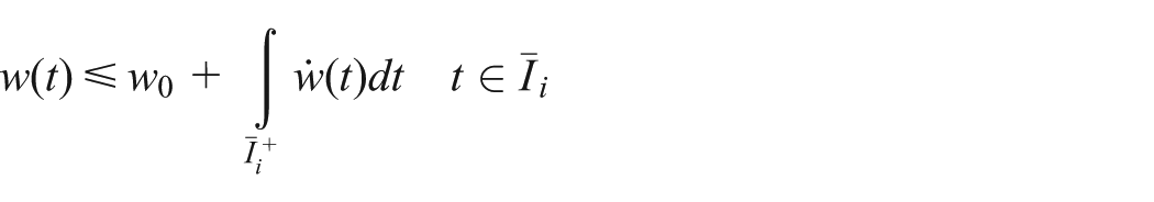
w(t) were uniformly bounded

Based on Lemmas 1 and 2, we can conclude that the solution trajectory $w(t)$ of system (3) crosses above and below the equilibrium point $w_0$ or converges to the equilibrium point $w_0$ . Without loss of generality, assume ${\phi }_0<w_0$ , so we can assume that the trajectories of equation (3) was illustrated (Figure 5).

Figure 5.

The solution trajectories of FAST TCP model (3).

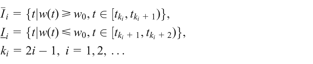
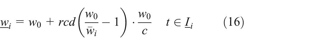
As shown in Figure 5, define oscillating period $i$ : $I_i={\overline{I}}_i\cup I_i$ , where $I_0=I_0=[-max(R(t)),t_1)$

$$\begin{array}{c}{\overline{I}}_i=\{t|w(t)\ge w_0,t\in [t_{k_i},t_{k_i+1})\},\hfill \\ {\underset{¯}{I}}_i=\{t|w(t)\le w_0,t\in [t_{k_i+1},t_{k_i+2})\},\hfill \\ k_i=2i-1,i=1,2,\dots \hfill \end{array}$$

For each period $i$ , clearly, we have

$$w(t_{k_i})=w(t_{k_i+1})=w_0,\stackrel{·}{w}(t_{k_i})>0,\stackrel{·}{w}(t_{k_i+1})<0$$

(5)

Define upper and lower bounds

$$\begin{array}{c}{\overline{w}}_i\in {\overline{W}}_i=\{w|w\ge \underset{t\in {\overline{I}}_i}{max}(w(t))\}\hfill \\ {\underset{¯}{w}}_i\in {\underset{¯}{W}}_i=\{w|\mathrm{cd}\le w\le \underset{t\in I_i}{min}(w(t))\},{\underset{¯}{w}}_0=\mathrm{cd}\hfill \end{array}$$

(6)

$${\overline{I}}_i^{+}=\{t|\stackrel{·}{w}(t)>0,t\in {\overline{I}}_i\},{\underset{¯}{I}}_i^{-}=\{t|\stackrel{·}{w}(t)<0,t\in {\underset{¯}{I}}_i\}$$

(7)

$${\stackrel{̑}{I}}_i={[t_{k_i},t_{k_i}+t\prime ),}_i=[t_{k_i+1},t_{k_i+1}+t\prime )$$

(8)

where $t\prime =w_0/c$ .

Hence, from equation (3), we have

$$w(t)=w(t_{k_i})+\underset{t_{k_i}}{\overset{t}{\int }}\stackrel{·}{w}(t)\mathrm{dt},t\in {\overline{I}}_i$$

From equation (6), only consider $\stackrel{·}{w}(t)>0$ . Then, we have

$$w(t)\le w_0+\underset{{\overline{I}}_i^{+}}{\int }\stackrel{·}{w}(t)\mathrm{dt}t\in {\overline{I}}_i$$

For $\underset{t\in {\overline{I}}_i}{min}(w(t))=w_0$ , from Lemma 1(b), we get

$$w(t)\le w_0+\underset{{\overline{I}}_i^{+}}{\int }\mathrm{rcd}(\frac{w_0}{w(t-R_c)}-1)\mathrm{dt},t\in {\overline{I}}_i$$

(9)

In a similar way, we get

$$w(t)\ge w_0+\underset{{\underset{¯}{I}}_i^{-}}{\int }\mathrm{rcd}(\frac{w_0}{w(t-R_c)}-1)\mathrm{dt}t\in {\underset{¯}{I}}_i$$

(10)

From equations (8) and (9), if we get the bounds of the $w(t-R_c)$ and the integral interval length, we can calculate the upper and lower bounds. In order to get the bounds of $w(t-R_c)$ , we should discuss the relation between $(t-R_c)$ and the integral interval. The following lemmas give this relation and the appropriate integral interval length.

Theorem 1

For each period $i$ :

• (a) If $t\in {\overline{I}}_i^{+}$ , then $t-R_c\in {\underset{¯}{I}}_{i-1}$ ; if $t\in {\underset{¯}{I}}_i^{-}$ , then $t-R_c\in {\overline{I}}_i$ .

• (b)  ${\overline{I}}_i^{+}\subseteq {\stackrel{̑}{I}}_i,{\underset{¯}{I}}_i^{-}\subseteq {\underset{⌣}{I}}_i$ , ${\stackrel{̑}{I}}_i$ , and ${\underset{⌣}{I}}_i$ were the appropriate integral intervals.

• (c) If $t\in {\underset{¯}{I}}_i$ , then $t-R_c\in I_i$ ; if $t\in {\overline{I}}_i$ , then $t-R_c\in {\underset{¯}{I}}_{i-1}\cup {\overline{I}}_i$ .

• (d) If $t\in {\stackrel{̑}{I}}_i$ , then $t-R_c\in {\underset{¯}{I}}_{i-1}$ ; if $t\in {\underset{⌣}{I}}_i$ , then $t-R_c\in {\overline{I}}_i$ .

Proof

• (a) Proof by mathematical induction.

When $i=1$ , by Lemma 1(c), $t\in {\overline{I}}_1^{+}$ implies $\stackrel{·}{w}(t)\ge 0,w(t)\ge w_0$ and $w(t-R_c)<w_0$ . Hence, when $t\in {\overline{I}}_1^{+}$ , we have $t-R_c\in {\underset{¯}{I}}_0$ ; similarly, when $t\in {\underset{¯}{I}}_1^{-}$ , we have $t-R_c\in {\overline{I}}_1$ . Hence, when $i=1$ , this conclusion was true.

Assume this conclusion was true for $i-1$ $(i>1)$ , therefore, if $t\in {\overline{I}}_{i-1}^{+}$ , then $t-R_c\in {\underset{¯}{I}}_{i-2}$ and if $t\in {\underset{¯}{I}}_{i-1}$ , then $t-R_c\in {\overline{I}}_{i-1}$ . The latter implies if $t\in {\underset{¯}{I}}_{i-1}$ , we have $w(t-R_c)\ge w_0$ . From equation (2), we have $R_c=w(t-R_c)/c\ge w_0/c$ . So, we have

$$t_{k_{i-1}+2}-t_{k_{i-1}}=t_{k_i}-t_{k_{i-1}}>R_c\ge \frac{w_0}{c}$$

(11)

We next prove that this conclusion was true for $i(i>2)$ . First, we prove that if $t\in {\overline{I}}_i^{+}$ , then $t-R_c\in {\underset{¯}{I}}_{i-1}$ .

Proof by contradiction

Suppose $t\in {\overline{I}}_i^{+}$ and $t-R_c\notin {\underset{¯}{I}}_{i-1}$ , by equation (5) and Lemma 1(c), $t\in {\overline{I}}_i^{+}$ implies $w(t-R_c)<w_0$ . Therefore, we can assume $t\in {\overline{I}}_i^{+}$ and $t-R_c\in {\underset{¯}{I}}_{i-2}$ . Hence, we have

$$t_{k_i}-t_{k_{i-1}}<t-(t-R_c)=R_c$$

(12)

From equation (2), we have $R_c=w(t-R_c)/c<w_0/c$ . Hence, equation (11) contradicts equation (10). Furthermore, $t\in {\overline{I}}_i^{+}$ and $t-R(t)\in {\underset{¯}{I}}_{i-h},h=3,4,...$ can lead to a similar contradiction. Second, we prove that if $t\in {\underset{¯}{I}}_i^{-}$ , then $t-R_c\in {\overline{I}}_i$ . Similarly, suppose $t\in {\underset{¯}{I}}_i^{-}$ and $t-R_c\notin {\overline{I}}_i$ .

By equation (5) and Lemma 1(c), $t\in {\underset{¯}{I}}_i^{-}$ implies $w(t-R_c)>w_0$ . Hence, we can assume $t\in {\underset{¯}{I}}_i^{-}$ and $t-R_c\in {\overline{I}}_{i-1}$ , and then there must exist a time ${\tau }_2$ that

$${\tau }_2\in {\underset{¯}{I}}_i^{-}\mathrm{and}{\tau }_2-R_c\in {\overline{I}}_{i-1}$$

(13)

From aforementioned conclusion, we have $t\in {\overline{I}}_i^{+}$ and $t-R_c\in {\underset{¯}{I}}_{i-1}$ . Hence, there must exist a time ${\tau }_1$

$${\tau }_1\in {\overline{I}}_i^{+},{\tau }_1-R_c\in {\underset{¯}{I}}_{i-1}$$

(14)

Hence, from equations (12) and (13), we have ${\tau }_1<{\tau }_2$ , ${\tau }_1-R_c>{\tau }_2-R_c$ . This contradicts Lemma 3(b). Furthermore, $t\in {\underset{¯}{I}}_i^{-}$ and $t-R_c\in {\overline{I}}_{i-h},h=2,3,...$ can lead to a similar contradiction. These contradictions prove that Theorem 1(a) was true.

• (b) Set $t_{k_i}=\tilde{t}-R_c$ and ${\tilde{I}}_i=[\tilde{t}-R_c,\tilde{t}]$ . From equation (2), $R(\tilde{t})=w(t_{k_i})=w_0/c$ , hence $\tilde{t}=t_{k_i}+w_0/c$ and ${\tilde{I}}_i={\hat{I}}_i$ .

If $\tilde{t}\ge t_{k_i+1}$ , then ${\overline{I}}_i^{+}\subseteq {\overline{I}}_i\subseteq {\tilde{I}}_i={\hat{I}}_i$ . If $\tilde{t}<t_{k_i+1}$ , from equation (4) and ${\overline{I}}_i$ , we have $w(\tilde{t})>w_0$ and $w(\tilde{t}-R_c)=w_0$ and from Lemma 1(c), we have $\stackrel{·}{w}(t\prime )<0$ . Furthermore, from Lemma 3(b), for $t\in [\tilde{t},t_{k_i+1})$ , we have $w(t)>w_0$ and $w(t-R_c)\ge w_0$ and by Lemma 1(c), we have $\stackrel{·}{w}(t)<0$ for $t\in [t\prime ,t_{k_i+1})$ . This implies ${\overline{I}}_i^{+}\subseteq {\tilde{I}}_i={\stackrel{̑}{I}}_i$ .

Similarly, we have $I_i^{-}{\subseteq }_i$ . (c, d) from (a), there must exist a time $t_{k_i+1}$ and $t_{k_i+1}-R(t_{k_i+1})\in [t_{k_i},t_{k_i+1})$ . From Lemma 3(b), we have $t\in {\underset{¯}{I}}_i$ and $t-R_c\ge t_{k_i+1}-R(t_{k_i+1})\ge t_{k_i}$ . Hence, we conclude that if $t\in {\underset{¯}{I}}_i$ , then $t-R(t)\in I_i$ .

Similarly, we can also obtain other conclusions of (c, d). From Theorem 1, we can calculate the following upper and lower bounds and its iterative relation.

Lemma 3

For each periodic interval $I_i$

$${\overline{w}}_i=w_0+\mathrm{rcd}(\frac{w_0}{{\underset{¯}{w}}_{i-1}}-1)·\frac{w_0}{c}t\in {\overline{I}}_i$$

(15)

$${\underset{¯}{w}}_i=w_0+\mathrm{rcd}(\frac{w_0}{{\overline{w}}_i}-1)·\frac{w_0}{c}t\in {\underset{¯}{I}}_i$$

(16)

Proof

From equation (8) and Theorem 1(b), we have

$$w(t)\le w_0+\underset{{\stackrel{̑}{I}}_i}{\int }\mathrm{rcd}(\frac{w_0}{w(t-R_c)}-1)\mathrm{dt}t\in {\overline{I}}_i$$

(17)

From Theorem 1(d), we have $\underset{t\in {\stackrel{̑}{I}}_i}{min}w(t-R_c)=\underset{(t-R_c)\in {\underset{¯}{I}}_{i-1}}{min}w(t-R_c)={\underset{¯}{w}}_{i-1}$ . Based on Lemma 1(b), we substitute ${\underset{¯}{w}}_{i-1}$ into equation (16) and get the inequality

$$w(t)\le w_0+\mathrm{rcd}(\frac{w_0}{{\underset{¯}{w}}_{i-1}}-1)·\frac{w_0}{c},t\in {\overline{I}}_i$$

(18)

From equations (5) and (17), we get ${\overline{w}}_i$ , see equation (14). Similarly, we get ${\underset{¯}{w}}_i$ .

Stability analysis

In this section, we acquire the trajectory bounds of the FAST TCP model and its iterative equation and obtain the same global stability conditions as the existing conclusions. Then, we improve the calculation method for the trajectory bounds and acquire the less conservative trajectory bounds and the global stability conditions.

Theorem 2

If $\gamma d/T<1$ and $\alpha >0$ , then the FAST TCP (3) was globally stable.

Proof

From Lemma 4, we conclude that if ${\underset{¯}{w}}_1>{\underset{¯}{w}}_0$ , then the sequence of upper–lower bounds converge to $w_0$ and the FAST TCP (3) was globally stable. ⁴

Substituting ${\underset{¯}{w}}_0=\mathrm{cd}$ into equation (14), we obtain

$${\overline{w}}_1=w_0+\mathrm{rcd}(\frac{w_0}{{\underset{¯}{w}}_0}-1)·\frac{w_0}{c}=w_0(1+r\alpha /c)$$

(19)

Substituting equation (18) into equation (15), we get

$${\underset{¯}{w}}_1=w_0+\mathrm{rcd}(\frac{w_0}{{\overline{w}}_1}-1)·\frac{w_0}{c}=w_0-\frac{r^2\alpha d{w}_0}{c+r\alpha }$$

(20)

Substituting ${\underset{¯}{w}}_0=\mathrm{cd},w_0=\mathrm{cd}+\alpha$ and equation (19) into ${\underset{¯}{w}}_1>{\underset{¯}{w}}_0$ , we get

$$r(1-\mathrm{rd})\alpha >c(r^2{d}^2-1)$$

(21)

From equation (20), we have the following:

if $1-\mathrm{rd}>0$ and $\alpha >-c(\mathrm{rd}+1)/r$ , then ${\underset{¯}{w}}_1>{\underset{¯}{w}}_0$ , where $r=\gamma /T$ .

if $1-\mathrm{rd}<0$ and $\alpha <-c(\mathrm{rd}+1)/r$ , then ${\underset{¯}{w}}_1>{\underset{¯}{w}}_0$ .

Considering $\alpha >0$ , we get that if $\gamma d/T<1$ and $\alpha >-c(\mathrm{rd}+1)/r>0$ , the FAST TCP (3) was globally stable.

Obviously, the global stability condition of Theorem 2 was the same as the existing conclusion in Chen et al. ² and Wang et al. ³

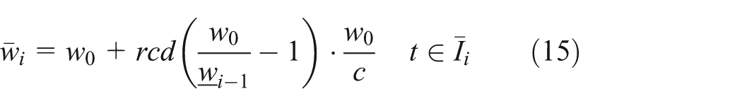
In equation (14), we substitute the lower bounds ${\underset{¯}{w}}_{i-1}$ into the trajectory of $w(t-R_c)$ in the integral interval $\hat{I}$ , so we obtained the conservative upper bounds ${\overline{w}}_i$ . In order to get less conservative trajectory bounds and global stability conditions, we define the new upper and lower bounds ${\underset{¯}{w}}_i\in {\overline{W}}_i$ and ${\underset{¯}{w}}_i\in {\underset{¯}{W}}_i$ . As shown in Figure 6, we subdivide the integral interval ${\stackrel{̑}{I}}_i$ as follows

${\stackrel{̑}{I}}_i=\bigcup _{j=0}^n{\stackrel{̑}{I}}_{i,j},n>0$ , where ${\stackrel{̑}{I}}_{i,0}=[t_{k_i},t_{k_i}+w_0/c-n\Delta )$ , and ${\stackrel{̑}{I}}_{i,j}=[t_{k_i}+w_0/c-j\Delta ,t_{k_i}+w_0/c-(j-1)\Delta )$ , $j=1,2,...,n$ , $\Delta =d/m$ and $\mathrm{nd}/m<w_0/c$ .

Figure 6.

Subdivision the integration interval.

The following lemmas give the improved method to calculate less conservative trajectory bounds.

Lemma 4

• (a) If $t\in {\stackrel{̑}{I}}_{i,j}$ and $j>0$ , then $t-R(t)>t_{k_i}-j\Delta$ .

• (b)  $\underset{t\in I_i}{max}(\stackrel{·}{w}(t))\le r(w_0-\underset{¯}{w}{\prime }_i)$ .

• (c)  $\underset{t\in {\stackrel{̑}{I}}_{i,j}}{min}(w(t-R(t)))\ge w_0-j\Delta r(w_0-\underset{¯}{w}{\prime }_{i-1})$ .

Proof

• (a) From Theorem 1(d), if $t\in {\stackrel{̑}{I}}_{i,j}$ and $j>0$ , then $t-R_c\in {\underset{¯}{I}}_{i-1}$ .

Hence, $R_c=w(t-R_c)/c<w_0/c$ . From ${\stackrel{̑}{I}}_{i,j}$ , we have $t-R_c>t_{k_i}+w_0/c-j\Delta -R_c>t_{k_i}-j\Delta$ .

• (b) From Theorem 1(c), we have $\underset{t\in I_i}{min}(w(t-R_c))=\underset{¯}{w}{\prime }_i$ ; from equation (7), $\underset{t\in I_i}{min}(w(t))=\underset{¯}{w}{\prime }_i$ , and by Lemma 1(c), we have

$$\begin{array}{c}\multicolumn{1}{c}{\stackrel{·}{w}(t)=r(\alpha -w(t)(1-\frac{\mathrm{cd}}{w(t-R_c)}))}\\ \le r(\alpha -\underset{¯}{w}{\prime }_i(1-\frac{\mathrm{cd}}{\underset{¯}{w}{\prime }_i}))\hfill \\ =r(\alpha -\underset{¯}{w}\prime +\mathrm{cd})=r(w_0-\underset{¯}{w}{\prime }_i),t\in {\underset{¯}{I}}_i\hfill \end{array}$$

Hence, $\underset{t\in I_i}{max}(\stackrel{·}{w}(t))\le r(w_0-\underset{¯}{w}{\prime }_i)$ .

• (c) From equation (2), when $t=t_{k_i}+w_0/c$ , we have $t-R_c=t_{k_i}$ and $w(t-R_c)=w_0$ .

From (a), when $t\in {\stackrel{̑}{I}}_{i,j}$ and $j>0$ , $t-R_c>t_{k_i}-j\Delta$ . From (b), $w(t)$ cannot increase in any interval of length $j\Delta$ by more than $j\Delta r(w_0-\underset{¯}{w}{\prime }_{i-1})$ . Hence, we can calculate that $\underset{t\in {\stackrel{̑}{I}}_{i,j}}{min}(w(t-R_c))\ge w_0-j\Delta r(w_0-\underset{¯}{w}{\prime }_{i-1})$ .

$$\mathrm{Set}\underset{¯}{w}{\prime }_{i-1,j}=max(\underset{¯}{w}{\prime }_{i-1},w_0-j\Delta r(w_0-\underset{¯}{w}{\prime }_{i-1}))$$

(22)

From equation (8) and Lemma 1(b), we have

$$\begin{array}{c}\multicolumn{1}{c}{w(t)\le w_0+\underset{{\stackrel{̑}{I}}_{i,0}}{\int }\mathrm{rcd}(\frac{w_0}{\underset{¯}{w}{\prime }_{i-1}}-1)\mathrm{dt}}\\ +\sum _{j=1}^n\underset{{\stackrel{̑}{I}}_{i,j}}{\int }\mathrm{rcd}(\frac{w_0}{\underset{¯}{w}{\prime }_{i-1,j}}-1)\mathrm{dt}\hfill \end{array}$$

(23)

An immediate consequence was as follows.

Lemma 5

$$\begin{array}{c}\multicolumn{1}{c}{\overline{w}{\prime }_i=w_0+\mathrm{rcd}(\frac{w_0}{\underset{¯}{w}{\prime }_{i-1}}-1)(w_0/c-n\Delta )}\\ +\sum _{j=1}^{\eta }\mathrm{rcd}(\frac{w_0}{\underset{¯}{w}{\prime }_{i-1,j}}-1)\Delta \hfill \end{array}$$

(24)

where $\underset{¯}{w}{\prime }_{i-1,j}=max(\underset{¯}{w}{\prime }_{i-1},w_0-j\Delta r(w_0-\underset{¯}{w}{\prime }_{i-1}))$ , $j=1,2,\dots ,n,\Delta =d/m$

$$\underset{¯}{w}{\prime }_i=w_0+\mathrm{rcd}(\frac{w_0}{\overline{w}{\prime }_i}-1)(w_0/c),{\underset{¯}{w}}_0^{\prime }=\mathrm{cd}$$

(25)

Comparing Lemma 6 to Lemma 4, clearly, we have $\overline{w}{\prime }_i\le {\overline{w}}_i,\underset{¯}{w}{\prime }_i\ge {\underset{¯}{w}}_i$ , and we obtained the less conservative trajectory bounds. Hence, we can get the following improved global stability conditions.

By calculating the maximum growth rate within the time-delay interval, the corresponding lower conservative bound at each moment was calculated by backward method, and the lower conservative solution trajectory bound was calculated by continuous integration method.

As shown in Figure 7, by calculating the maximum growth rate within the delay interval, the corresponding lower bound of lower conservatism at each moment was calculated by backward method, and the lower conservative solution trajectory bound was calculated by continuous integration method.

Figure 7.

Subdivision of integral interval.

Theorem 3

The FAST TCP (3) was global stability for

$$\alpha +\mathrm{rcd}(\frac{w_0}{{\overline{w}}_1}-1)(\frac{w_0}{c}-n\Delta )+\sum _{j=1}^n\mathrm{rcd}(\frac{w_0}{{\overline{w}}_{1,k_j}}-1)\Delta >0$$

(26)

where $r=\gamma /T$ , ${\overline{w}}_1=w_0+r\alpha (w_0/c-n\Delta )+\sum _{j=1}^n\mathrm{rcd}\left(\frac{j\Delta r\alpha }{w_0-j\Delta r\alpha }\right)\Delta$

$${\overline{w}}_{1,k_j}=w_0-j\Delta r(w_0-{\overline{w}}_1),j=0\dots n,\Delta =d/m$$

Proof

From Lemma 6, we concluded that if $\underset{¯}{w}{\prime }_1>\underset{¯}{w}{\prime }_0$ , then the sequence of upper–lower bounds converged to $w_0$ , and the FAST TCP (3) was globally stable. ⁴

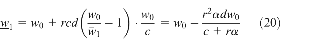
From $\mathrm{rd}<m/n$ , we have $w_0-j\Delta r(w_0-\underset{¯}{w}{\prime }_{i-1})>\underset{¯}{w}{\prime }_{i-1}$ , so we have $\underset{¯}{w}{\prime }_{i-1,j}=w_0-j\Delta r(w_0-\underset{¯}{w}{\prime }_{i-1})$ . Substituting $\underset{¯}{w}{\prime }_0=\mathrm{cd}$ and ${\underset{¯}{w}}_{0,j}=w_0-j\Delta r\alpha$ into equation (23), we obtained

$$\overline{w}{\prime }_1=w_0+r\alpha (w_0/c-\eta \Delta )+\sum _{j=1}^{\eta }\mathrm{rcd}\left(\frac{j\Delta r\alpha }{w_0-j\Delta r\alpha }\right)\Delta$$

(27)

Substituting equation (26) into equation (24), we get

$$\begin{array}{c}\multicolumn{1}{c}{\overline{\underset{¯}{w}}{\prime }_1=w_0+\mathrm{rcd}(\frac{w_0}{\overline{w}{\prime }_1}-1)(w_0/c-\eta \Delta )}\\ +\sum _{j=1}^{\eta }\mathrm{rcd}(\frac{w_0}{\overline{w}{\prime }_{1,k_j}}-1)\Delta \hfill \end{array}$$

(28)

Substituting $\underset{¯}{w}{\prime }_0=\mathrm{cd},w_0=\mathrm{cd}+\alpha$ and equation (27) into $\underset{¯}{w}{\prime }_1>\underset{¯}{w}{\prime }_0$ , we get the conclusion of this theorem.

Remark 1

From Theorem 2, if $\gamma d/T<1,\alpha >-c(\mathrm{rd}+1)/r>0$ , then

$$\alpha +\mathrm{rcd}(\frac{w_0}{{\overline{w}}_1}-1)·\frac{w_0}{c}>0$$

From Lemma 6, we know $\overline{w}{\prime }_1\le {\overline{w}}_1$ . Hence, we have

$$\alpha +\mathrm{rcd}(\frac{w_0}{\overline{w}{\prime }_1}-1).\frac{w_0}{c}\ge \alpha +\mathrm{rcd}(\frac{w_0}{{\overline{w}}_1}-1)·\frac{w_0}{c}>0$$

Therefore, if the global stability condition of Theorem 2 was true, then the condition of Theorem 3 was true.

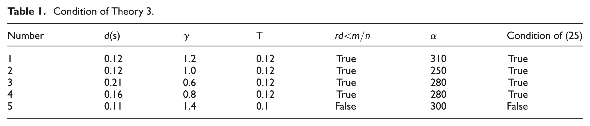
It can also be seen from the derivation of equation (25; Theorem 3) that, if $n=0$ , the global stability condition (25) of Theorem 3 degenerates to the same as that of theorem. According to equation (25), under the condition $\eta \Delta =\eta d/\kappa <w_0/c$ , the higher the values of $n$ and $m$ , the higher the accuracy and the lower the conservatism. Now, assume c = 250,000 packets/s. When the condition $\eta d/\kappa <w_0/c$ was satisfied, we set n = 10 and m = 12, respectively, according to the parameters $c,d$ , $\gamma$ , $\alpha$ , $T$ . The right-hand side of the global stability condition inequality (25) of Theorem 3 was calculated, which is shown in Table 1.

Table 1.

Condition of Theory 3.

Number	$d$ (s)	$\gamma$	T	$\mathrm{rd}<m/n$	$\alpha$	Condition of (25)
1	0.12	1.2	0.12	True	310	True
2	0.12	1.0	0.12	True	250	True
3	0.21	0.6	0.12	True	280	True
4	0.16	0.8	0.12	True	280	True
5	0.11	1.4	0.1	False	300	False

From Table 1, there exist $\gamma ·d/T>1$ and $\alpha >0$ such that the condition of Theorem 3 was satisfied, but the condition of Theorem 2 was not satisfied.

Hence, we can conclude that the global stability condition of Theorem 3 was less conservative than the condition of Theorem 2.

Simulation and conclusions

We present a set of NS-2 simulation results to illustrate the validity of the conditions for the global stability of FAST TCP presented in Theorem 3. The code of Chen et al. ² and Wang et al. ³ for simulation of FAST TCP was slightly modified to disable the algorithm of Multiple Increase (MI). Note that $w(t)>\mathrm{cd}$ , so we do not disable the algorithm of MI. In addition to this, the simulation was performed for the same environment considered in Chen et al. ² and Wang et al. ³

Figure 8 shows the validity of condition (25) for the cases that the relevant parameters were selected according the parameters of Table 1 with larger propagation delay.

Figure 8.

Simulation validation of proposed condition (25), where c = 2000 Mb/s, $\alpha =500$ .

The simulation environment was UBUNTU7.04 + NS2.31, adopting the single-link single-path network topology structure as shown in Figure 8. Assuming the buffer size of the link end was 80,000 packets. The link adopts the DropTail algorithm, and the size of each packet was 1000 bytes. Considering the small parameter setting of propagation delay in the simulation environment of Chenmin. ⁷ In this article, propagation delay d of the simulation environment was set to be greater than 0.1 s. Now assume bottleneck link bandwidth c = 250,000 packets/s. The values of $\alpha$ , $\gamma$ , $d$ , and $T$ are shown in Table 1.

By the condition formula (25) of the stability of Theorem 3, given the parameters of $n,m$ , $c$ , $d$ , $\gamma$ , $T$ , $\alpha$ , we can calculate the left side value of formula (25). If the above value was greater than 0, the stability condition of Theorem 3 was satisfied, which are shown in numbers 1–4 of Table 1, and the simulation results show that the FAST TCP system (3) can converge to the equilibrim as shown in Figure 3. From the number 5 of Table 1, when the global stability condition of Theorem 3 was not satisfied, the simulation results show that the FAST TCP system (3) cannot converge to the equilibrium point as shown in Figure 8.

The theoretical computation and NS-2 simulation results demonstrate that the proposed global stability conditions of FAST TCP possess a larger stability region of parameters in contrast to the existing conditions described in Chenmin. ⁷

Related research

FAST TCP^1,2 was proposed by Steven H Low et al. of network laboratory of California Institute of Technology, and FAST TCP^1–3 was a new type of transmission control protocol proposed for the next generation of high-speed networks of high performance networks with high speed, long delay, and large capacity, and its global stability had attracted the attention of scholars.^4–9 Tan et al. ⁹ and Koo et al. ¹⁷ studied the global stability of the FAST system, but it simplified the case of time delay and time variation. In Koo et al. ¹⁷ and Choi et al., ¹⁸ the Lyapunov–Razumikhin stability theorem and LMI method were used to obtain the global stability condition with lower conservativeness than that in Tan et al., ⁹ where time delay and time variation were not simplified. Choi et al. ¹⁹ studied the global asymptotic stability of FAST system considering other mixed flows, proving that the system was globally asymptotically stable when the flow of other mixed flows was less than half of the bottleneck link bandwidth, and gave the conditions for the global asymptotic stability of the system, when the flow of other mixed flows was more than half of the bottleneck link bandwidth. Choi et al. ²⁰ studied the possible complex nonlinear phenomena of FAST system when the algorithm lost stability using nonlinear theory. The direction of Hopf bifurcation and the stability of periodic solution were determined using the central manifold theorem. In Tan et al., ⁹ by studying the changing law of the trajectory boundary of the solutions of nonlinear time-varying and time-delayed FAST systems, a lower conservative global stability condition was obtained than in Tan et al. ⁹ and Koo et al. ¹⁷ In order to improve the stability of the system, Choi et al. ²¹ proposed an improved FAST algorithm, which took into account the size of the sending window of the previous round-trip cycle before deciding the window adjustment strategy. Due to the historical information taken into account by the improved strategy, the system stability was improved. Meanwhile, the conditions for the global exponential stability of the improved FAST system were given in Choi et al. ²¹ Through theoretical analysis and experimental simulation, Koo et al. ²² verified that the improved FAST system in Choi et al. ²¹ had better stability than the original FAST system in Tan et al. ⁹ and Koo et al., ¹⁷ but the response speed was slower, and further improved algorithm was proposed according to the characteristics of the above two systems.^9,17,19 The performance of the improved system was between the above two systems. The global stability condition of the improved system was given using Lyapunov–Razumikhin theorem. Choi et al. ²¹ analyzed the global stability of network congestion control time-delay model in Koo et al. ²² by analyzing and solving the trajectory boundary. However, in the process of analysis, Koo et al. ²² did not consider the time-varying characteristics of the time delay, but used the average round-trip delay to approximate the time-varying time delay.

Since the time delay was fixed, the bound of the time delay term could be taken within the accurate time-delay range, and then the nonlinear function was characterized by monotone decline. When calculating the upper bound, the trajectory of the time delay term within the whole time-delay range can be replaced with a minimum lower bound value. Therefore, the trajectory bounds with a large conservative property were obtained. In view of the above defects in choosing the protocol parameter guidance scheme, in this article, a FAST TCP network congestion control model considering the window update period parameter $T$ and exponential smoothing filter was established. In addition, the stability condition of the model was analyzed. An improved guidance scheme to select appropriate protocol parameters was proposed to ensure the stability of FAST system according to controller gain parameter $\gamma$ , window update period $T$ , propagation delay $d$ , and link bandwidth $c$ .

Conclusions and future research work

Although this article gives the global stability condition of FAST TCP, which was less conservative than the existing conclusion, the theoretical calculation, however, shows that the range can only be changed from the original $\gamma d/T\in (0,1)$ to $\gamma d/T\in (0,1.2)$ . The simulation results showed that when $\gamma d/T=1.3$ , the FAST TCP system still showed stability. Therefore, for this kind of nonlinear and time-delay model, how to find a more effective control theory method and further reduce the conservatism of its global stability conditions theoretically is the next step that we need to study. At the same time, the improved stability conditions of FAST TCP proposed in this article were all verified under the NS-2 simulation environment. There was still a big gap between the simulation environment and the complex transmission environment in the actual network. How to integrate the improvement stability conditions proposed in this article and apply it to the real network was the next step for us to study.