
Abstract
Since speed sensors are not as widely used as GPS devices, the traffic congestion level is predicted based on processed GPS trajectory data in this article. Hidden Markov model is used to match GPS trajectory data to road network and the average speed of road sections can be estimated by adjacent GPS trajectory data. Four deep learning models including convolutional neural network, recurrent neural network, long short-term memory, and gated recurrent unit and three conventional machine learning models including autoregressive integrated moving average model, support vector regression, and ridge regression are used to perform congestion level prediction. According to the experimental results, deep learning models obtain higher accuracy in traffic congestion prediction compared with conventional machine learning models.
Keywords
Introduction
With the improvement of living standards, the vehicle possession per capita continues to grow. As a result, pressure on urban transportation system is increasing. 1 The transportation system is a complicated system which is composed of pedestrians, cars, and roads. The system is affected by many stable and unstable factors. The stable factors include the number of road lanes, road grades, and urban areas, and the unstable factors include road construction and traffic control. For cities with incomplete urban layouts, it is effective to alleviate traffic congestion by improving road infrastructure. In contrast, it is efficient to solve the problem by predicting traffic congestion precisely and carrying out proper deployment for cities with mature urban layouts.
Quality and quantity of data with traffic information will influence a lot in performing traffic congestion prediction. Traffic information collected by fix detection sensors is accurate. Therefore, most studies on traffic congestion prediction are based on these data. However, the quantity of fixed detection devices is not enough to cover most part of road networks because of their high cost. For those roads without fixed sensors, traffic congestion is hard to predict. Nevertheless, with the roaring growth of vehicles with GPS, it is cost effective to use GPS floating car devices to gather traffic information. GPS trajectory data are more comprehensive, in real time and in a large scale. 2
Nonetheless, the data measured by the GPS equipment show deviation. An important step to process raw GPS trajectory data is to match them to the actual road network. Accurate prediction results of traffic congestion level can provide residents with reasonable decision support, save residents’ time, and improve road utilization and traffic capacity. Consequently, the efficiency and security of the transportation network will be improved by predicting traffic congestion accurately.
In this article, a procedure shown in Figure 1 is proposed to perform traffic congestion level prediction based on GPS trajectory data. The main ideas of this article are as follows: (1) first, the GPS trajectory data are matched to roads, and experimental road networks are selected according to map matching results; (2) the average driving speed of road networks is calculated by the results of map matching step and then the calculation result is converted to time sequences and temporal–spatial image; (3) the convolutional neural network (CNN) and the recurrent neural network (RNN) series models are used to predict the average driving speed of the road networks; (4) finally, the traffic congestion levels are classified according to the traffic congestion level standard.

An illustration of the traffic congestion prediction based on GPS trajectory data.
The article is organized as follows: section “Introduction” presents the introduction. Section “Literature review” presents a literature review, which summarizes the related map matching technology and traffic flow prediction research. Section “Map matching” discusses hidden Markov model (HMM)-based map matching algorithm and analyzes the matching results. Section “Traffic congestion prediction based on deep neural network” discusses four deep neural network models used in this article, namely, CNN, RNN, long short-term memory (LSTM), and gated recurrent unit (GRU). Section “Analysis of results” analyzes the experimental results. Section “Conclusion” summarizes the research and points out the future research direction.
Literature review
Map matching technology research
The map matching algorithms can be roughly divided into four categories: map matching algorithm based on geometric information, road topology information, probability information, and integrated information.
In terms of geometric information, a map matching model is proposed in Li and Huang
3
to measure the degree of geometric similarity between candidate routes and GPS trajectory. A genetic model is utilized which takes into consideration both path cost and shape similarity between the observed paths and GPS trajectories.
4
The
In terms of road topology information, an algorithm based on the topological relationship of road traffic network on the existing map matching model was proposed. 5 The topological relationship of the road network was used in this model to determine the range of candidate road sections and performs map matching based on historical trajectory database. The disadvantage is that only the distance between the GPS points and the candidate roads is considered, and the driving direction is not taken into account. Topological ordering and a local search tree were utilized in Rahmani and Koutsopoulos 6 to implement online map matching. However, map matching models based on topology information only take road connectivity into consideration. For GPS trajectories with many anomaly points, this kind of model will not perform well.
In terms of probability information, HMM that adopts direction, speed, and α-trimmed mean filters to reduce the scale of candidate sets was proposed by Mohamed et al. 7 Another HMM-based map matching model is proposed to use Viterbi algorithm to generate a partial route with a high confidence. 8 A cellular-based trajectory map matching SnapNet system that showed a difference with the actual road network was introduced by Mohamed et al. 9 Probability-based map matching models have a high accuracy. The models tend to generate complete matching trajectories because they take all the states into account, but they are trained by a large amount of data. When the amount of training data is little, the probability-based model will also mismatch many points.
In terms of integrated information, a method which fuses multiple kinds of traffic information (i.e. speed and direction) and takes the global effect into consideration was utilized by Hu et al. 10 In addition, a historical model was used to estimate the historical traffic speed and current surrounding traffic speed based on temporal and spatial analyses. The influential factor based on spatial distribution of the middle location between two continuous GPS coordinates on low-frequency GPS trajectories was considered by the spatial and temporal conditional random field (ST-CRF) map matching model. 11 Similar to most existing studies, both the consistency of driving direction and the temporal–spatial accessibility between two consecutive GPS coordinates are considered in the ST-CRF model. The model is basically an HMM map matching model based on Viterbi algorithms. 12 Map matching models considering integrated information are complex and time-consuming, so they are not online models.
In this article, an HMM-based map matching algorithm is adopted to match the GPS trajectory points to road. Considering the fact that the HMM-based map matching model is a global algorithm and its accuracy is higher than that of other local algorithms, HMM is used to implement map matching based on GPS trajectory data.
Traffic flow prediction research
The main idea of this article is to use the deep neural network to predict the average speed of selected road networks and then classify the traffic congestion level according to the traffic congestion level standard. Therefore, the traffic flow forecast will be reviewed below.
In the field of traffic flow prediction, research methods can be basically divided into two categories: parametric and nonparametric approaches.
Parametric approaches are based on empirical data and theoretical assumption to decide the model parameters, such as Kalman filter models and autoregressive integrated moving average (ARIMA)-based models, which are classical time series models. 13 A model with one parameter was proposed to predict traffic condition efficiently. 14 The autoregressive model was combined with other prediction methods to optimize prediction performance. The autoregressive model proposed in Davoodi et al. 15 is used for traffic flow prediction.
The advantage of parametric methods includes (1) low model complexity and (2) ease of implementation. However, the traffic network is complex and shows nonlinear and stochastic change, and the parametric approaches cannot handle the uncertainty well. The prediction performance of the parametric methods will be influenced by many external factors in the transportation system. Otherwise, parametric models are usually based on prior knowledge in specific field in practice.
For nonparametric approaches, large-scale training data are necessary to build the model structure. The common nonparametric models include support vector regression (SVR), k-nearest neighbor (KNN), artificial neural network (ANN), and the Bayesian network model. 16 A model taking singular point probabilities into account was proposed by Liu et al. 17 A prediction model which combined ANN with root mean square error (RMSE) was utilized by Qian et al. 18 The radial basis function (RBF) model taking the analysis of chaotic characteristics into account was implemented to predict traffic flow by Chen. 19 Compared with conventional nonparametric approaches, deep learning based parametric models can build higher dimensional space to match the real solution space.
RNNs and their variants can extract some sequence features in the input data. While the driving speed in road networks has temporal characteristics, RNN models such as RNN, 20 LSTM 21 and GRU (Cho et al., 2014) 22 can be considered to predict traffic flow. A deep bidirectional long short-term memory (DBL) model proposed in Wang et al. 23 is utilized to extract feature. A LSTM-based model which utilized attention mechanisms to perceive long-term intensive traffic flow and improves the long-term memory of LSTM was proposed by Yang et al. 24 Nonetheless, transportation system has both temporal and spatial characteristics, but the RNN series models focus only on the temporal features.
Traffic flow data can be represented to a space-time matrix and can be converted to image, so the CNN model can be used to extract features from the image and learn temporal-spatial characteristics from traffic flow. The CNN model was used to predict traffic flow. The prediction results were converted to corresponding congestion level. Then the accuracy is calculated based on the congestion prediction. 25 The experimental results show that the CNN model has the highest accuracy when the mean square error (MSE) value is the lowest.
In the following, the taxi GPS data will be preprocessed by the HMM-based map matching algorithm. According to the map matching result, the experimental roads are selected and the average speed of the experimental road sections is calculated.
Map matching
Taxi GPS trajectory data preprocessing
The raw GPS trajectory data are the GPS trajectory data of taxis from the time period of 3–30 August 2014 in Chengdu, China. As shown in Table 1, the data include such fields as taxi number, time stamp, and the longitude and latitude of the vehicle at that moment. In addition, the original data also include information whether or not passenger is carried. The GPS trajectory data are disordered in the time dimension and some data are missing. In addition, for the convenience of experiment, only a part area of Chengdu and about 2000 taxis are selected to conduct the experiments, so raw data need to be preprocessed.
Taxi GPS trajectory data field.

Data supplementation and sorting
The raw data are unordered on the timeline, so the GPS trajectory data for each vehicle per day need to be sorted by time stamp. In addition, the original data include the taxi GPS trajectory data of Chengdu from the time period of 3–30 August 2014. However, the data on the dates 7, 13, and 17 of August are missing. According to the analysis of traffic flow characteristics, 24 the missing 3-day data of 2000 taxis can be replaced by another 2000 taxis’ GPS trajectory data on 14th, 20th, and 24th of August.
Data filtering
The selected area is part of the urban area of Chengdu. The longitude ranges from 103.94 and 104.2, and the latitude ranges from 30.57 to 30.75. Therefore, some taxi GPS track points may be outside the map. In this article, the GPS track points outside the selected area are excluded, and the sequence with such kind of points is divided into many parts.
HMM-based map matching algorithm
The HMM is a probability model that can be used to process time series. The HMM describes a random sequence of randomly generated unobservable states from a hidden Markov chain. Then a corresponding observation based on each state is generated to form a process of observing random sequences. A sequence of random states generated by hidden Markov chains is called a sequence of states; each state corresponds to an observation and a sequence of random observations based on this is called an observation sequence.
As shown in Figure 2, the sequence

HMM-based map matching model.
Figure 2 presents the illustration of the HMM-based map matching model in this article. Each GPS point (e.g.
However, it will cause a large deviation in practical applications by taking the observation probability into consideration solely. Such problems as winding, turning around, and unreachability during the time interval arise. Therefore, the reachability of adjacent candidate points should be considered. In the HMM, this can be represented by the transition probability of two adjacent candidate points. Then the hidden Markov chain is built.
In this article,

For
Given an observed GPS trajectory point, the projection of this point in all road segments in the road network can be regarded as its candidate points. The GPS positioning error can be approximated as a Gaussian distribution with a mean of 0,
26
and the observation probability of
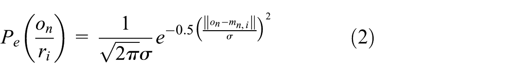
where
Trajectory built by two adjacent candidate points may not be a normal driving trajectory. Taking the condition into consideration, the probability of driving from a candidate point to another candidate point is regarded as the transition probability. It is shown in Newson and Krumm 27 that the correct travel path distance is often similar to the large arc distance of adjacent GPS points. Therefore, the transition probability can be described as
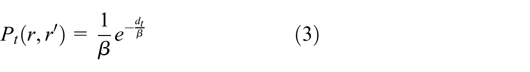
where
The process of the hidden Markov map matching algorithm is shown in Table 2.
Map matching algorithm based on HMM.

HMM: hidden Markov model.
Map matching result analysis
The performance of the HMM-based map matching model is mainly influenced by two factors.
First, if the time interval in a GPS trajectory is long, GPS points are likely to be mismatched to other nearby roads. Figure 3 shows the map matching result. The time intervals in the trajectory in a yellow box in Figure 3 range from 10 to 319 s. Those points with a short sampling interval tend to match well, while some points with a long sampling interval tend to be mismatched to a wrong road. The green matched points in a yellow box in Figure 3 change from a main road to another road when the red true GPS points maintain its tendency.

Map matching result with large sampling time interval points.
Second, if there are many roads with high similarity to GPS trajectory, GPS points also tend to be wrongly matched to other routes. Figure 4 shows the map matching result of a trajectory and Figure 5 shows an enlarged view of the yellow box in Figure 4. In Figure 5, it can be estimated that the blue road should be the proper matching road, but red GPS points are mismatched to the roads which green points are in. One possible reason is that the wrongly matched roads’ shapes are similar to the proper road and they are closer to red GPS points. This phenomenon happens frequently in wrongly matching results.
Map matching result with similar road in the road network.

Enlarged view in map matching result with similar road in the road network.
Road network selection
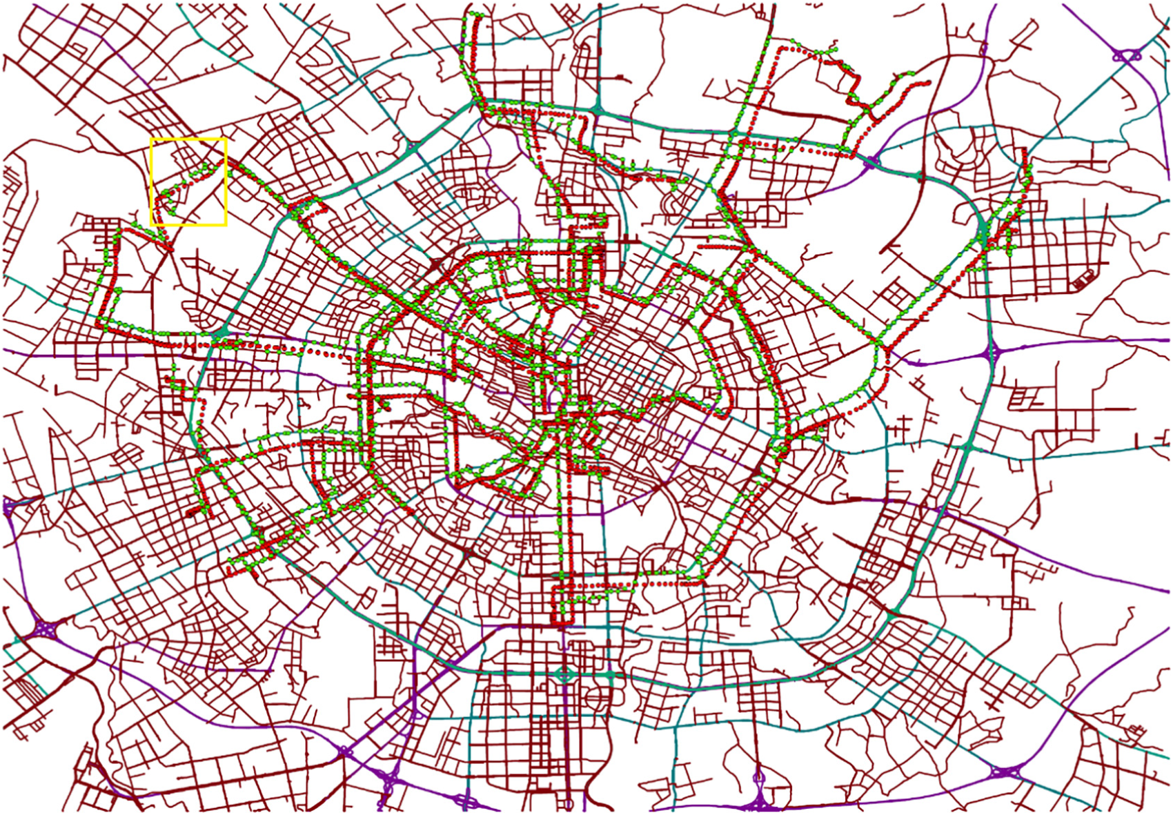
The complete road network in Chengdu is complicated. There are many roads with high similarity in some areas, which has a great influence on the performance of map matching. If GPS points are mismatched to some roads, the average speed calculated by map matching results will be unreliable. Therefore, it is necessary to select road networks to avoid the problem mentioned above. The selected road networks should have fewer roads similar to nearby roads.
The road networks selected in this article are shown in Figure 6. The number of roads in Network 1 is 385 and that in Network 2 is 588. As shown in Figure 6, the red thick roads represent Network 1 and the green thick roads represent Network 2. There are fewer roads with similar degrees around the selected network and these two road networks are moderately dense.

Road network selection.
Calculating the average speed of road section
Since it is necessary to predict the congestion level of selected road networks at a certain moment in the future, the average speed of selected road networks should be predicted first. Then, according to the prediction results, the congestion grade of selected road networks can be classified by the traffic congestion level classification standard of Chengdu. Therefore, the congestion of selected road networks at certain moment in the future can be predicted. This is actually a time series prediction problem. The input of the prediction model is the average driving speeds in the past. The output of the prediction model is the predicted traffic congestion levels in the future. For the purposes of predicting traffic congestion of selected road networks, the average driving speed of selected road networks is calculated by the following steps in this article. First, map matching is performed on a certain number of taxis’ GPS trajectory data. The average driving speed of a road in selected road networks can be calculated using formula (4)

where
In the next section, the CNN, RNN, LSTM, and GRU models will be introduced to perform the prediction of the average driving speed in selected road networks. Then the traffic congestion level classification will be carried out according to the traffic operation level classification standard. 28 Finally, the experimental results will be analyzed.
Traffic congestion prediction based on deep neural network
CNN model building
The deep learning model has been widely used in computer vision and image recognition, and has achieved remarkable results. 29 The traffic flow of the road networks can be transformed into a space–time image. In this image, temporal dimension features are related to a road’s traffic information with the change of timeline. Spatial dimension features are related to the traffic flow information in a time stamp among all roads. The CNN can learn the temporal and spatial characteristics of the selected road network well. Therefore, the traffic congestion level of selected road networks at a certain moment in the future can be predicted by the CNN model.
The procedure to predict average driving speed in road networks is shown in Figure 7. The input of the CNN model is a space–time image. After extracting the temporal–spatial features of the input, prediction is made by a fully connected layer.

Illustration of the CNN structure in this article.
Figure 8 presents the form of the input image. In Figure 8,


The input of the CNN model.
In this article, we select two road networks. For Network 1, the resolution of the input image is
The output of the convolution and pooling layer can be described as

where
The input of convolution and pooling layer of layer

After extracting the features, the

Finally, the vector is converted to the output of the model through a fully connected layer. Therefore, the output of the model can be described as

where
RNN model building
RNN model
RNNs can learn the sequence information and features in the data. 20 The traffic flow changes with time, so it has temporal characteristics. Therefore, it is reasonable to use a time series prediction model to predict traffic flow. The RNN and its two variants LSTM and GRU models are used to predict the average driving speed in selected road networks in this article.
The network structure of the RNN model used in this article is shown in Figure 9, where

Illustration of the RNN model structure.
Figure 10 shows the time series input of the RNN model and its variants. The time series input in Figure 10 can be described as

where
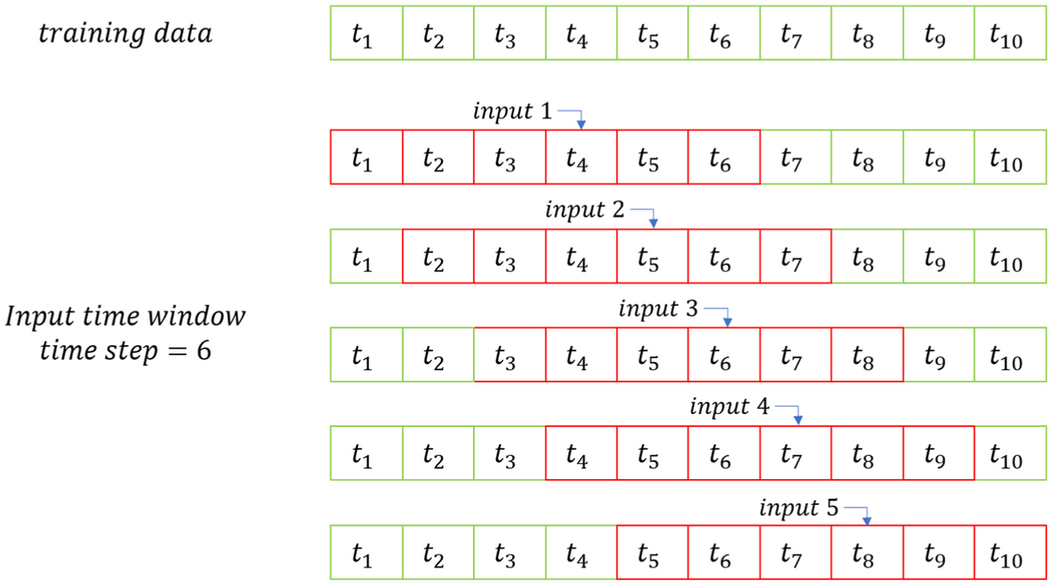
Time series input of the RNN model.
The calculation in the hidden layer can be described as

where
The calculation of the output layer can be described as

LSTM model
The LSTM model is an improved model based on the RNN model. 21 The main improvement is that gate structure is added in the hidden layer.
Figure 11 presents the inner structure in a hidden layer. A hidden layer contains three gates, an input gate, a forgetting gate, and an output gate. The input of a hidden layer includes the output of the previous hidden layer, the recorded cellular information, and the input at the current time point. The input gate plays a role in selectively recording the input information into the cell state. The function of the forgetting gate is to forget some state information in the cell. The function of the output gate is to selectively output the result of the hidden layer.

Illustration of the LSTM hidden unit structure.
The calculation in the hidden layer is described by formulae (13)–(18), where
The calculation of the forgetting gate

where
The input gate

The candidate cell information

where the tanh function is an activation function.
The cell information

The output gate

The final output

GRU model
The GRU model is a variant of the LSTM model (Cho et al., 2014). The GRU model combines the input gate and the forgetting gate into an update gate, which incorporates the cell state and the hidden state.
The inner structure in the GRU hidden unit is shown in Figure 12. A GRU hidden unit contains two gates: reset gate and update gate. The reset gate determines how much current input is combined with previous memory information. The update gate determines how much previous memory information is retained. When the reset gate is set to 1 and the update gate is set to 0, the GRU model is equivalent to the RNN model.

Illustration of the GRU hidden unit structure.
The update gate

where
The reset gate

where
The hidden layer output


where
Compared with the LSTM model, the GRU model has a simpler internal structure, so its training speed will be faster than that of LSTM when dealing with large training datasets.
The structures of the LSTM and GRU models applied in our article are similar to that of the RNN model shown in Figure 9. Both the GRU and LSTM models have three hidden layers.
Time series of average driving speed is regarded as the input of the RNN, LSTM, and GRU models. The temporal characteristics of the input sequence can be learned by the RNN model and its variants. The spatial and temporal characteristics of the input can be learned by the CNN model.
The prediction results of three conventional machine learning models and four deep neural network models mentioned above are analyzed below.
Analysis of results
In this article, the GPS data of nearly 2000 taxis in 28 days are used as the dataset, where about 80% data (22 days) in the dataset are used as the training set and about 20% data (6 days) as the test set.
In terms of the experiments, four different lengths of input time window units are selected to predict the average driving speed in selected road networks. The description of experimental tasks is shown in Table 3. The time window unit in the input is set as the average driving speed in selected road networks within 5 min.
Experimental tasks.

The raw GPS data are collected by taxis in Chengdu. The classification standard shown in Table 4 is made by Chengdu Transportation Department. Therefore, we adopt the standard in Table 4 to classify the road states. 28
Classification of traffic congestion level of Chengdu in the main road.

In this article, four deep learning models including the CNN, RNN, LSTM, and GRU models and three conventional machine learning models including ARIMA, SVR, and ridge regression models are used for prediction. Four performance indexes including MSE, mean absolute error (MAE), RMSE, and accuracy are used in this article. MSE, MAE, and RMSE are calculated based on the predicted speed and the calculated speed after map matching. Accuracy is calculated based on the congestion level of the predicted speed and the congestion level of the calculated speed after map matching.
Three conventional machine learning models are used to perform prediction in this article. Table 5 gives the performance of ARIMA, SVR, and ridge regression. As shown in Table 5, with the growth of the length of input time window units, the MSE, MAE, and RMSE of the three models are all increased. When the input length of units is set at 6, the three models obtain the minimum MSE, MAE, and RMSE values compared with the input lengths of 8, 12, and 18. The phenomenon shows that conventional machine learning models perform better in short-term prediction than long-term prediction in our experiments. However, the MSE values of conventional models range from 116.87 to 240.33 and the accuracy ranges from 75.92% to 83.59%, which is not as good as the performance of deep learning models. One of the reasons may be that traffic flow contains both linear and nonlinear features, but conventional machine learning models cannot learn nonlinear features well from the input. In the short term, linear features influence the tendency of traffic flow more seriously than nonlinear features. In the long term, nonlinear features play a more important role. Consequently, conventional machine learning models perform not very well in our study.
The performance of the ARIMA, SVR, and ridge regression models.
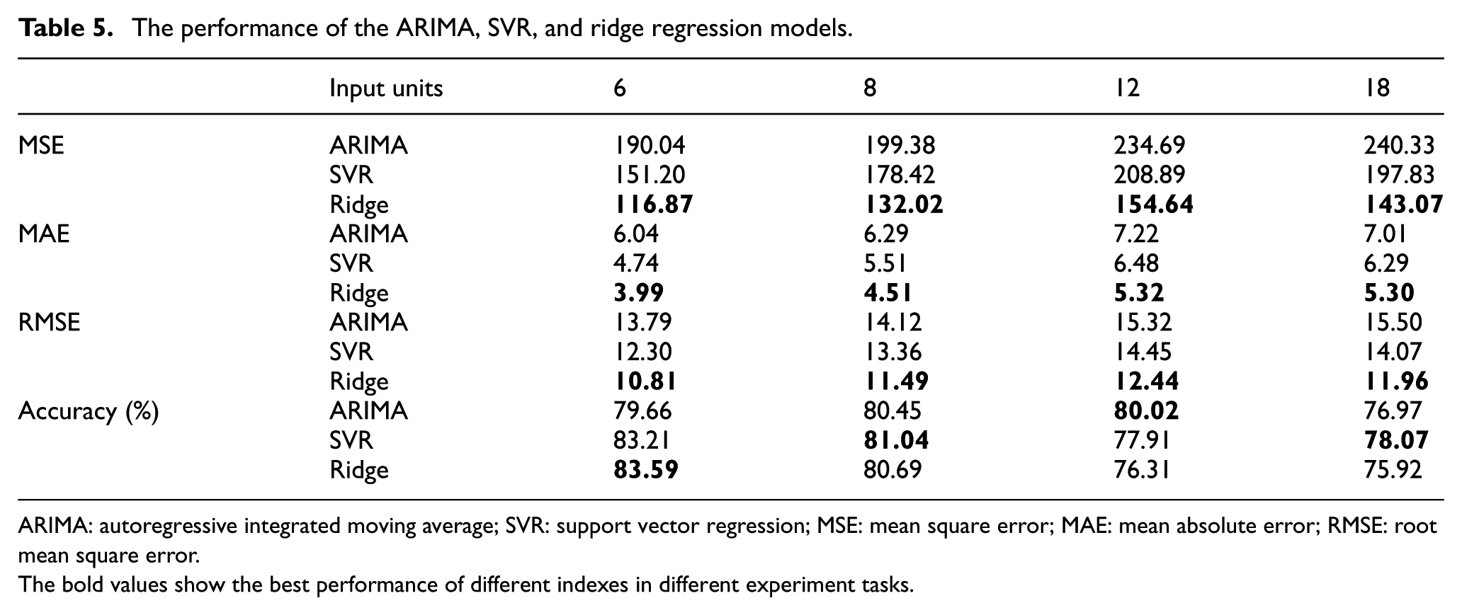
ARIMA: autoregressive integrated moving average; SVR: support vector regression; MSE: mean square error; MAE: mean absolute error; RMSE: root mean square error. The bold values show the best performance of different indexes in different experiment tasks.
In addition, four deep learning models are utilized to realize prediction. Table 6 gives the hyperparameters of the CNN, RNN, LSTM, and GRU models.
Hyperparameters of the CNN, RNN, LSTM, and GRU models.

CNN: convolutional neural network; RNN: recurrent neural network; LSTM: long short-term memory; GRU: gated recurrent unit.
The hyperparameters shown in Table 6 are decided by the experimental results shown in Figures 13–17. Figure 13 shows the loss curves of the RNN model when the batch size is set at 128, 256, and 512, while the input length is set at 6, 8, 12, and 18, respectively. It can be seen from Figure 13(a) and (c) that the RNN model has the lowest MSE values when the batch size is 128 and it has the highest MSE values when the batch size is 512 and the training epoch is 500. It can be seen from Figure 13(b) and (d) that the RNN model is trained the best when the batch size is 128 and the RNN model is trained the worst when the batch size is 256. Therefore, the batch size of 128 is used for the RNN model and its variants in the remaining experiments.

The loss curves of the RNN model: (a) input time window length = 6, (b) input time window length = 8, (c) input time window length = 12, and (d) input time window length = 18.

The loss curves of the CNN model (filter number = 32, kernel size = (3, 3)): (a) input time window length = 6,(b) input time window length = 8, (c) input time window length = 12, and (d) input time window length = 18.

The loss curves of the CNN model (filter number = 32, kernel size = (5, 5)): (a) input time window length = 6, (b) input time window length = 8, (c) input time window length = 12, and (d) input time window length = 18.

The loss curves of the CNN model (batch size = 128, kernel size = (3, 3)): (a) input time window length = 6, (b) input time window length = 8, (c) input time window length = 12, and (d) input time window length = 18.

The loss curves of the CNN model (batch size = 128, filter number = 32): (a) input time window length = 6, (b) input time window length = 8, (c) input time window length = 12, and (d) input time window length = 18.
Figure 14 presents the loss curves of the CNN model when the batch size is set at 128, 256, and 512, the filter number is 32, and the kernel size is
Figure 16 shows the loss curves of the CNN model when the batch size is set at 128, the filter number is 32, 64, and 128, and the kernel size is
Figure 17 shows the loss curves of the CNN model when the batch size is 128, the filter number is 32, and the kernel size is set at
It is shown that the CNN and RNN series models perform well in our study. The CNN model can learn the temporal–spatial features from the input. The RNN model and its variants can learn temporal features well from the short-term input and the long-term input. Table 7 gives the performance of the four models. It can be seen from Table 7 that the CNN model has the lowest MSE, MAE, and RMSE values than the RNN series models in most of the situations. It is proposed that the CNN model is able to learn temporal–spatial features from the space–time image. However, the accuracy of the CNN model is lower than that of the RNN series models in most of the situations. The reason may be that some prediction values (e.g. 19.5 km/h) have small gaps with real values (21 km/h), but they are classified into different congestion levels. In addition, with the increment of the length of the input units, the MSE value of the CNN model drops quickly. This shows that the CNN model tends to perform well in long-term traffic flow prediction. For the RNN model, the MSE, MAE, and RMSE values drop when the length of the input units is less than 12 and rises when the length of the input units is bigger than 12. In contrast, the MSE, MAE, and RMSE values of the LSTM and GRU models drop with the increment of the length of the input time window units. The minimum MSE, MAE, and RMSE values are achieved with an input length of 18. This indicates that the RNN model performs better in short-term prediction than long-term prediction. The GRU and LSTM models are good at predicting long-term time sequences.
The performance of the CNN, RNN, LSTM, and GRU models.
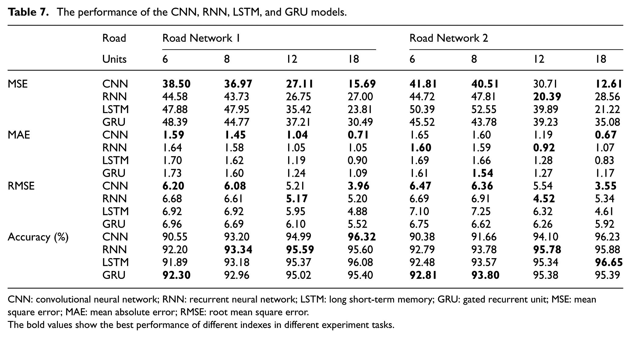
CNN: convolutional neural network; RNN: recurrent neural network; LSTM: long short-term memory; GRU: gated recurrent unit; MSE: mean square error; MAE: mean absolute error; RMSE: root mean square error.The bold values show the best performance of different indexes in different experiment tasks.
To sum up, conventional machine learning models perform well in short-term linear prediction, while deep learning models show their advantages in our study. Moreover, the CNN model is able to learn the temporal–spatial features from traffic flow space–time images and its prediction ability is no less than that of the RNN series models in our study. In addition, the RNN series models can learn temporal features from the time series input and perform well in time sequence prediction. The RNN model predicts well in short-term traffic flow prediction and its performance drops when the length of the time series input becomes long. By comparison, the LSTM and GRU models are able to perform well in predicting long-term series.
Conclusion
Deep neural network is widely used to solve a variety of problems, including traffic flow prediction and traffic congestion prediction. However, the existing research on traffic flow prediction and traffic congestion prediction is mostly based on off-the-shelf traffic flow data gathered by fixed detection sensors. A large number of detection devices are required to collect such kind of data. Therefore, research in this field can only be applied to those roads where detection sensors are installed. As a result, the application range of the research is limited.
The experiments in this article are based on GPS trajectory data which can be easily obtained by floating cars. Our study can expand the application range of traffic flow prediction. The procedure of our methods includes the following steps. First, a map matching algorithm based on the HMM model is used in this article to preprocess taxi GPS trajectory data. After the map matching process, the average driving speed in selected road networks at each moment can be calculated. The calculation results are regarded as the input of the deep neural networks. The prediction models are used to predict the average driving speed of the road networks at a moment in the future. According to the traffic congestion level classification standard, the prediction results are classified into the corresponding congestion grade. In this article, four deep learning models and three conventional machine learning models are used for prediction. However, ARIMA, SVR, and ridge regression do not perform as good as deep learning models. In terms of deep neural networks, the RNN, LSTM, and GRU models show similar performance in these experiments. The GRU and LSTM models perform better in long-term prediction than the RNN model. In addition, the CNN model has the lowest MSE value compared with the RNN series models, which proves that it has the ability to learn the temporal and spatial characteristics in traffic flow space–time images.
There are still some shortcomings in this article and these will be considered as the research directions of our future study. First, the HMM-based map matching model can be replaced by some state-of-the-art map matching algorithms. Second, this article only uses the data from the time period of 3–30 August 2014. The GPS trajectory data of 2000 taxis in 28 days are still insufficient. It can be considered to use more GPS data. Finally, the network structure of the CNN model can be improved to enhance the performance.
Footnotes
Handling Editor: Muhammed Ali Imran
Declaration of conflicting interests
The author(s) declared no potential conflicts of interest with respect to the research, authorship, and/or publication of this article.
Funding
The author(s) disclosed receipt of the following financial support for the research, authorship, and/or publication of this article: The authors would like to thank the National Natural Science Foundation of China (Grant No. 61104166).