Sage Journals: Discover world-class research

Abstract

To solve the problem that high-redshift and broad emission lines weaken the quasar discovery and observation severely, a new redshift calculation method based on piecewise Gaussian fitting is proposed. The denoised and normalized spectrum is divided into two regions, peak and non-peak, by mean square error threshold segmentation first. Then, the non-peak region spectrum is applied to fit the continuous spectrum, removal of which gains access to the residual spectrum. And, the peak of each segment in the residual spectrum is precisely fitted by single-peak Gaussian fitting to replace the original multi-peak Gaussian fitting. Finally, through matching the accurate peak value with the stationary template, the redshift value is acquired. Compared with traditional methods, the method proposed improves the precision of continuous spectrum fitting and redshift calculation. The effectiveness and accuracy of this method have been verified by experiments based on the Sloan Digital Sky Survey data.

Keywords

Quasars redshift Gaussian fitting Sloan Digital Sky Survey

Introduction

Quasars are distant objects with very high redshift, which is caused by the space expansion between the quasars and the earth. More than 200,000 quasars are mainly observed by the Sloan Digital Sky Survey (SDSS). The observed quasars spectra are with redshifts ranging from 0.056 to 7.085.^1,2 And, the astronomical data volume at different wavebands grows dramatically with the continuous sky surveying research by the large space-based and ground-based telescopes, such as SDSS, Large Sky Area Multi-Object Fibre Spectroscopic Telescope (LAMOST), FIRST, and Two Degree Field (2dF) Redshift Survey. The existing and forthcoming astronomical database volume is too large to apply traditional analysis technics.³ In the next decade, the ongoing project FAST (Five-hundred-meter Aperture Spherical radio Telescope) will face this severe challenge inevitably. Redshift is the most important physical parameter of quasar, which can be characterized by the relative difference between the observed and static wavelengths (or frequency) of an object.⁴ The redshift can be calculated as

z = \frac{λ'}{λ} - 1

(1)

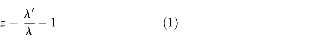
where $λ$ is the static wavelength, $λ'$ is the observation wavelength, and z is the redshift.

At present, the research works on the quasars’ redshift identification are mainly concerned on the template matching method. The earliest and most classic algorithm of template matching is the cross-correlation method proposed by Tonry and Davis.⁵ Glazebrook improved Tonry’s method by replacing the individual templates by simultaneous linear orthogonal templates.⁶ This improvement eliminates the mismatch between templates and data effectively and provides a better error estimation.^5–7 However, the PCAZ can only be applied to measure tiny redshifts due to the wavelength range restriction of the orthogonal templates. And, these methods usually require high integrity of template combination.

Recently, machine learning algorithms have been applied to find quasars in astronomy. Neural network, K-means, K-neighborhood, Gaussian modeling, and many other methods have improved the redshift calculation accuracy and commutable range effectively.^8–13 But, the identification methods based on spectral are very sensitive to the accuracy of characteristic line. However, the quasar has wide and less emission line, which results in the difficulty of extracting characteristic lines.^14,15 This article is aimed at improving the original automatic peaks identification and obtaining accurate characteristic lines.^1–3 And, the piecewise Gaussian fitting (PGF) divides the spectrum into different peaks and none-peaks areas. This method could be adapted to provide robust automatic redshifts for broad emission lines and large galaxy redshift. For the SDSS survey, there was a substantial improvement in the reliability of assigned redshifts and in the lowering of redshift uncertainties.

In the following sections, the spectral data used in this article and the spectral pretreatment is described in section “Data preparation.” In section “Characteristic lines extraction based on PGF,” the mean square deviation is used to classify the peak region where the characteristic line is located. This can not only avoid the broad spectrum problem when fitting the continuum but also identify each peak parameters one by one. In section “Redshift calculations and simulation verification,” PGF is used for computing the peak parameters and redshift values. Simulation results of the algorithm will be shown in section “Redshift calculations and simulation verification.” And, section “Conclusion” gives a conclusion of our research.

Data preparation

All the spectra in our experiment are from SDSS. SDSS is a major multi-filter imaging and spectroscopic redshift survey using a dedicated 2.5-m wide-angle optical telescope at Apache Point Observatory in New Mexico, USA. The survey will map in detail one-quarter of the entire sky with five broadband filters, determining the positions and absolute brightness of more than 100 million celestial objects. Data collection began in 2000, and the final imaging data release covers over 35% of the sky, with photometric observations of around 500 million objects and spectra for more than 3 million objects. The main galaxy sample has a median redshift of z = 0.1; there are redshifts for luminous red galaxies as far as z = 0.7 and for quasars as far as z = 5; and the imaging survey has been involved in the detection of quasars beyond a redshift z = 6. The spectra contain wavelengths covering the range 4000–9000 Å. The peak search method is sensitive to the noise level for noise peaks which are dominant in most low signal-to-noise ratio (SNR) cases. So, we selected stars with an average SNR > 5. And, the spectrum pre-processing is necessary in advance.

Spectral denoising

Consider the noise of the spectrum is similar to the white noise, so select the median filter to denoise it. Median filtering is a commonly used nonlinear smoothing filter, whose basic principle is that each point value of the spectral sequence is replaced by the mean value of all points in the sliding window. We use the median filter method to extract the continuous spectrum of the quasar spectrum. Sliding window size of 60 nm is selected after tons of experiments.^16,17 The filtering effect is shown in Figure 1.

Figure 1.

Spectrum (a) before and (b) after being filtered.

Continuous spectrum fitting

The extraction of the characteristic lines must take into account the influence of the continuum first. Since the presence of the continuum makes the true intensity of the spectrum line be obscured and cannot be accurately obtained, the continuum must be removed. There are many articles using filter technology to fit the continuum, but the quasars are broad emission galaxies, and it is often difficult to obtain the ideal fitting effect by the filter algorithm.

Aiming at the problem of the continuum fitting of quasars broad emission, the method of RMS (root mean square) error comparison is used to divide the spectrum into quasi-peak region and non-peak region. The regions greater than 3δ ( $δ$ is the variance of the spectrum) are divided into the peak regions, and other regions can be regarded as the non-peak regions. The whole continuous spectrum fitting is based on the spectral curve of the non-peak regions.¹ The specific strategy is calculating the RMS for the whole spectrum first and then delimiting the peak regions which are larger than the threshold 3δ. Then, the continuum spectrum quantic polynomial fitting is performed using the non-peak region data set. This avoids the problems that broad emission line cannot be handled by sliding windows, filter, and so on. Figures 2 and 3 show the process of obtaining the continuous spectrum using the obtained non-peak regions.

Figure 2.

Peak region division.

Figure 3.

Continuous spectrum.

The areas between each of the two asterisks in Figure 2 are the region where the broad emissions are located and are also the characteristic lines are located. As we know, these regions are difficult to be filtered out, which is a problem in the quasar spectral pre-processing. In fact, our purpose is to obtain continuous spectrum, so accurate peak location is not necessary temporarily. Therefore, the algorithm can only use the RMS error to obtain its approximate position and remove it.

The residual spectrum or the emission spectrum is obtained by subtracting the continuum from the denoised spectrum, as shown in Figure 4.

Figure 4.

Residual spectrum.

Characteristic lines extraction based on PGF

The Gaussian function is a normal distribution function. In the application, many of the SED (spectral energy distribution) patterns can be described by the Gaussian curve. Although the Gaussian curve is a nonlinear function, but its parameters have reasonable physical meaning. The method has some advantages in simplified calculation, quick computer programming, and fast dissemination.^18,19

There are a lot of methods for the peak position determination, which is also the characteristic spectrum wavelength acquisition. These include the derivative method, the Lorentz curve fitting method, and multi-peak simultaneous fitting method. However, one question that comes up frequently is the lower accuracy. The main reason is that we often calculate multiple peaks at the same time, because under the influence of noise and sky light, it is easy to get false peaks and the wrong peak positions. For redshift calculations, this inevitably generates errors or even erroneous results. In view of this, PGF is put forward using the results of variance segmentation. Each individual peak region is a single Gaussian distribution. The individual fitting in each region avoids the identification error introduced by multi-peaks and multi-parameters. Finally, the peak parameters such as the peak positions and wave width are getting more accurately, and redshifts can be calculated based on these. The Gaussian function can be expressed as

f (x) = H e^{- {[(x - c) / σ]}^{2}}

(2)

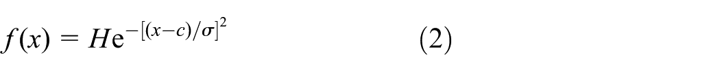
where c is the emission wavelength and H is spectral line relative intensity; c, H, and $σ$ are the parameters to be fitted. This function can be graphed with a symmetrical bell-shaped curve centered at the position c, with H being the height of the peak and σ controlling its width.

Assuming that there is a set of data ${x_{i}, y_{i}}, i = 1, 2, \dots, n$ for fitting, the purpose is on how we fit a Gaussian function to observed data points and determine the parameters, H, c, and σ exactly. The solution to the fitting problem is to employ the least-squares method to fit the data for Gaussian processing, which is deduced from noise model.¹⁸ Taking logarithm on both sides of equation (2)

\ln y_{i} = \ln H - \frac{{(x_{i} - c)}^{2}}{σ} = (\ln H - \frac{c^{2}}{σ}) + \frac{2 x_{i} c}{σ} - \frac{x_{i}^{2}}{σ}

(3)

Suppose

\ln y_{i} = z_{i}, \ln H - \frac{c^{2}}{σ} = b_{0}, \frac{2 c}{σ} = b_{1}, - \frac{1}{σ} = b_{2}

(4)

Equation (3) matrix form is expressed as

[\begin{matrix} z_{1} \\ z_{2} \\ ⋮ \\ z_{n} \end{matrix}] = [\begin{matrix} 1 & x_{1} & x_{1}^{2} \\ 1 & x_{2} & x_{2}^{2} \\ ⋮ & ⋮ & ⋮ \\ 1 & x_{n} & x_{n}^{2} \end{matrix}] [\begin{matrix} b_{0} \\ b_{1} \\ b_{2} \end{matrix}]

(5)

abbreviated as

Z = XB

(6)

Using the least squares principle, the generalized least squares solution of the matrix B is

B = (X^{T} X)^{- 1} X^{T} Z

(7)

The estimated parameters $H, c$ , and $σ$ can be obtained by equation (3). The fitting results are shown in Figure 5. There are three peaks in Figure 4. The parameter values are shown in Table 1.

Figure 5.

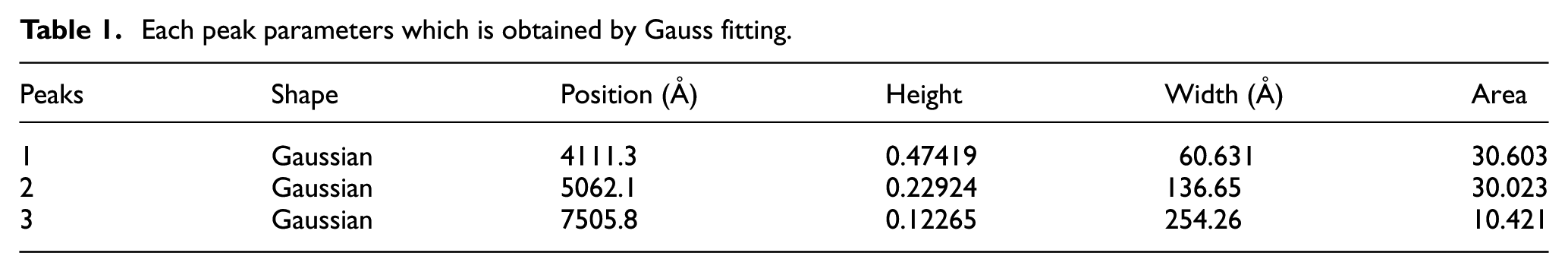
Fitting results of each peak: (a) peak 1, (b) peak 2, and (c) peak 3.

Table 1.

Each peak parameters which is obtained by Gauss fitting.

Peaks	Shape	Position (Å)	Height	Width (Å)	Area
1	Gaussian	4111.3	0.47419	60.631	30.603
2	Gaussian	5062.1	0.22924	136.65	30.023
3	Gaussian	7505.8	0.12265	254.26	10.421

Redshift calculations and simulation verification

Redshift calculation

After obtaining the characteristic spectrum, the red shift is calculated as follows:

Step 1. Do spectral pre-processing, denoise the spectrum by median filtering, and normalize the denoised spectrum to obtain the filtered spectrum $f_{R}$ .

Step 2. Calculate the RMS error $δ$ , divide the region greater than $3 δ$ into the peak regions, and divide the regions below $3 δ$ into the non-peak regions.

Step 3. Continuous spectrum removal operation. Using the result of step 2, the continuous spectrum is obtained by fitting the segmented region. And, subtract the continuous spectrum from the original spectrum to obtain the residual or the emission spectrum.

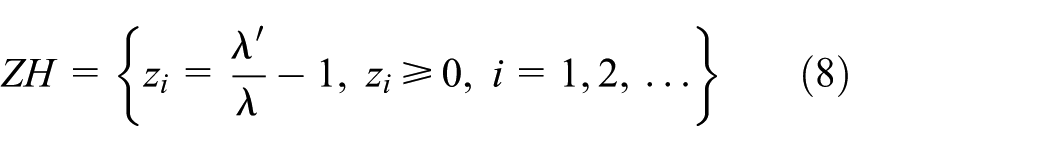
Step 4. Carry out Gaussian fitting on each peak region to obtain the exact peak value, which is also the emission line set $L' = {λ'_{i}, i = 1, 2, \dots, M}$ .

Step 5. Refer to the static template in Lewis and Ibata⁶ for redshift calculation. Suppose the template spectral characteristic wavelength set is $L = {λ_{i}, i = 1, 2, \dots, M}$ . Then, calculate the redshift candidate set

ZH = {z_{i} = \frac{λ'}{λ} - 1, z_{i} ⩾ 0, i = 1, 2, \dots}

(8)

Step 6. According to the calculated spectral characteristic line value, compared with the laboratory standard spectral line table, find the redshift and confirm the line.

The central wavelength of the spectral line can be obtained from the emission line set $L'$ , which is obtained from step 4. The SDSS website provides the laboratory emission line wavelength table and the emission weights as shown in Table 2 and Figure 6.

Table 2.

Eight most distinct emission lines of the composite quasar.

D	λ (Å)
Lyα	1216.25±0.37
CIV	1546.15±0.14
CIII	1905.97±0.12
MgII	2800.26±0.10
Hβ	4862.66^a
OIII	4960.36±0.22
OIII	5008.22±0.17
Hα	6564.93±0.22

Wavelength of Hβ is from Table 2 of Berk et al.²⁰

Figure 6.

The rest quasar spectrum template.

Using the information provided above, we can find the redshift value through the following process:

Sort the n spectrum characteristic lines from small to large according to the center wavelength and store them in the array $Λ$ .

Calculate the candidate redshift for each characteristic line. First, assume $Λ [i] (i = 1, 2, \dots, n)$ is the jth $(j = 1, 2, \dots, m)$ spectrum characteristic line on the wavelength table and then calculate the corresponding redshift value $z_{ij} (i = 1, \dots, n; j = 1, \dots, m)$ .

For the ith remaining line in $Λ [i], i = 1, 2, \dots, n$ , except for the jth one, use z_ij to calculate the spectrum line moving back central wavelength and compare them with the spectral line in Table 2. When the wavelength deviation is less than the specific threshold value k, we can confirm that this line is the corresponding spectrum in the standard table. Finally, store all the successful match line pairs into a set $Γ_{i}$ .

Calculate the weight sum of the $Γ_{i} (i = 1, 2, \dots, n)$ and then store them into S(i). Finally, extract the maximum weight sum $z = \max (s (i)), i = 1, 2, \dots, n$ . The spectrum final redshift is the z obtained in step 4, where the size of the threshold k depends on the accuracy of the spectral wavelength calibration, the center wavelength calculation error, spectral resolution, and other factors. Here, we take 15 Å, which refers to the calculation method in Song et al.¹

Simulation

In this section, we will present the performance of our PGF in terms of peak recognition and redshift calculation. All the data in our experiment are from Sloan Digital Sky Survey (SDSS). These data with the wavelength range from 4000 to 9000 Å. Figure 7 shows detailed information of the spectra SNR distribution in experiment. We can see that the low SNR will affect the extraction result.

Figure 7.

Signal to noise ratio distribution of the data set.

First, select 10 well SNR spectra, and their identification, peaks area, and redshift are shown in Figure 8. It can be seen that the ideal peak regions are obtained, and the redshift error values between the actual value and the predicted value are all within 0.02.

Figure 8.

Comparison results of the computing redshift and the segmentation and peaks of the first 10 spectral data.

The accuracy test is shown in Figure 9, the abscissa is the results obtained by the calculation, and the ordinate is the results provided by SDSS. The correct points of prediction are on the line of slope one, so we can see that the accuracy of redshift calculation is still quite satisfactory.

Figure 9.

Comparison of calculation results.

In order to compare the performance of redshift estimation by our PGF algorithm with that by the support vector regression (SVR) and backpropagation (BP) neural network, the 15 selected spectral redshift estimation values with these methods are shown in Table 3. The estimation $\overset{⌢}{Z}$ and estimation error $Δ Z$ —with the best $Δ Z$ as bold—are shown in Table 3. We can see clearly that most the estimation errors have been significantly decreased by adopting the new method. This demonstrates that our proposed approach is effective especially in high $\overset{⌢}{Z}$ situation.

Table 3.

Comparison of other methods and our integrated approach.

Real Z value		SVR	BP neural network		Conventional Gaussian fitting		PGF (our method)
Z	$\overset{⌢}{Z}$	$Δ Z$	$\overset{⌢}{Z}$	$Δ Z$	$\overset{⌢}{Z}$	$Δ Z$	$\overset{⌢}{Z}$	$Δ Z$
0.651527	0.663910	−0.01238	0.631172	0.02036	0.650151	0.00138	0.656044	−0.00452
0.693534	0.693876	−0.00034	0.693314	0.00022	0.693216	0.00032	0.693340	0.00019
0.772804	0.774815	−0.00201	0.778106	−0.00530	0.773116	–0.00031	0.777204	−0.00440
1.50811	1.52181	−0.0137	1.63025	−0.12214	1.63016	−0.12205	1.50941	–0.00130
1.61560	1.61905	–0.00345	1.67531	−0.05971	1.69874	−0.08314	1.61011	0.00549
1.62711	1.65353	−0.02642	1.62103	0.00608	1.69821	−0.0711	1.62333	0.00378
1.66049	1.71945	−0.05896	1.86328	−0.20279	1.84300	−0.18251	1.65618	0.00430
1.89174	1.8356	0.05614	1.85360	0.03813	1.98563	−0.09389	1.88509	0.00665
2.28985	2.20631	0.08354	2.15539	0.13446	2.01517	0.27468	2.29142	–0.00157
2.29095	2.31069	−0.01974	2.06736	0.22359	2.33698	−0.04603	2.28914	0.00181
2.30090	2.33648	−0.03558	2.41514	−0.11424	2.11714	0.18376	2.30855	–0.00765
3.03303	3.08963	−0.0566	3.59871	−0.56568	2.91876	0.11427	3.02980	0.00323
3.03465	3.06783	−0.03318	2.88631	0.14834	3.52375	−0.48919	3.02787	0.00678
3.04499	3.10624	−0.06125	3.17711	−0.13212	3.36515	−0.32016	3.03583	0.00916
4.01990	3.90153	0.11837	3.86315	0.15675	3.88963	0.13027	4.01936	0.00053

SVR: support vector regression; BP: backpropagation; PGF: piecewise Gaussian fitting

Conclusion

In this article, a new method to calculate the redshift is proposed based on the previous achievements. This method effectively overcomes the problems that the continuous spectrum cannot be fitted and the peaks cannot be obtained accurately. The root of these problems is the existence of the quasar broad emission line. Different from the previous method, PGF method obtains the peak area through threshold segmentation first and then obtains the characteristic spectral line using the gauss fitting in the peak area. The results show that this method is superior to the original method, which obtains the characteristic line at one time. With the progress of observation technology, more and more quasars will be observed, and our method can provide effective identification and calculation redshift strategy.

Footnotes

Handling Editor: Marcin Wozniak

Declaration of conflicting interests

The author(s) declared no potential conflicts of interest with respect to the research, authorship, and/or publication of this article.

Funding

The author(s) disclosed receipt of the following financial support for the research, authorship, and/or publication of this article: This work was supported by the Natural Science Foundation of Shandong Province (grant nos 2016ZRE2703, ZR2017PD010, and ZR2017PA004), the National Natural Science Foundation of China (grant no. 11803017), and the China Postdoctoral Science Foundation (grant no. 2016M600538).

ORCID iDs

Li Zhang

Fabao Yan

References

Song

Luo

Zhao

YH.

Searching QSO candidates and calculating their redshift from a flood of spectra. Spectrosc Spect Anal 2011; 31: 2578–2581 (in Chinese).

Richards

Myers

Peters

et al . Bayesian high-redshift quasar classification from optical and mid-IR photometry. Astrophys J. Epub ahead of print 28 July 2015. DOI: 10.1088/0067-0049/219/2/39.

Wang

Fan

Yang

et al . First discoveries of z>6 quasars with the DECam legacy survey and UKIRT Hemisphere Survey. Astrophys J 2017; 839: 27.

Zuo

XB.

The search for high-redshift quasars. Wuli 2016; 45: 1–10.

Tonry

Davis

. A survey of galaxy redshifts.1. Data reduction techniques. Astronom J 1979; 84: 1511–1525.

Glazebrook

Offer

Deeley

. Automatic redshift determination by use of principal component analysis — I: fundamentals. Astrophys J 1998; 492: 98–109.

Pan

Stellar atmospheric parameter estimation using Gaussian process regression. Month Not Roy Astronom Soc 2014; 447: 256–265.

Zhao

Luo

et al . Restricted Boltzmann machine: a non-linear substitute for PCA in spectral processing. Astronom Astrophys 2015; 576: A96.

Kuegler

Polsterer

Hoecker

Determining spectroscopic redshifts by using k nearest neighbor regression I. Description of method and analysis. Astronom Astrophys 2015; 576: A132.

10.

Liu

Duan

Luo

AL.

A method for redshift determination of quasars based on cross correlation. Spectrosc Spect Anal 2005; 25: 1155–1157 (in Chinese).

11.

Eigenbrod

Courbin

Meylan

et al . Microlensing variability in the gravitationally lensed quasar QSO 2237+0305 equivalent to the Einstein Cross II. Energy profile of the accretion disk. Astronom Astrophys 2008; 490: 933-9U75.

12.

Wang

et al . Searching QSO candidates and calculating their redshift from a flood of spectra. Acta Phys Sin 2016; 65: 56–64 (in Chinese).

13.

Tavasoli

Vasei

Mohayaee

The challenge of large and empty voids in the SDSS DR7 redshift survey. Astronom Astrophys 2013; 553: A15.

14.

Miller

Regier

et al . A Gaussian process model of quasar spectral energy distributions. In: 29th annual conference on neural information processing systems (NIPS), Montreal, Canada, 7–12 December 2015. La Jolla, CA: Neural Information Processing Systems (NIPS).

15.

Shen

Brandt

Richards

et al . The Sloan Digital Sky Survey reverberation mapping project: velocity shifts of quasar emission lines. Astrophys J 2016; 831: 80424648.

16.

Jian

Berk

DEV

. Fitting the continuum component of a composite SDSS quasar spectrum using CMA-ES. Eprint arXiv, 2013, https://arxiv.org/abs/1312.7356

17.

Matute

Marquez

Masegosa

et al . Quasi-stellar objects in the ALHAMBRA survey I. Photometric redshift accuracy based on 23 optical-NIR filter photometry. Astronom Astrophys 2012; 542: 201118111.

18.

Tian

Wang

et al . Short-term wind speed hybrid prediction model based on ARIMA and ESN. Acta Energ Solar Sin 2016; 37: 1603–1610 (in Chinese).

19.

Abramo

Strauss

Lima

et al . Measuring large-scale structure with quasars in narrow-band filter surveys. Month Not Roy Astronom Soc 2012; 423: 3251–3267.

20.

Yip

Connolly

Berk

DEV

et al . Spectral classification of quasars in the Sloan Digital Sky Survey: eigenspectra, redshift, and luminosity effects. Astronom J 2004; 128: 2603–2630.

The quasars’ redshift estimation method based on piecewise Gaussian fitting

Abstract

Keywords

Introduction

Data preparation

Spectral denoising

Continuous spectrum fitting

Characteristic lines extraction based on PGF

Redshift calculations and simulation verification

Redshift calculation

Simulation

Conclusion

Footnotes

Declaration of conflicting interests

Funding

ORCID iDs

References