
Abstract
Particle filtering algorithm has found an increasingly wide utilization in many fields at present, especially in non-linear and non-Gaussian situations. Because of the particle degeneracy limitation, various resampling methods have been researched. The estimation process of particle filtering algorithm is a series of weighted calculation processes, which can be regarded as weighted data fusion. This article proposed an improved particle filtering algorithm combining with different rank correlation coefficients to overcome the shortcomings of degeneracy. By simulating iteration operation in MATLAB, it discovers that the proposed algorithm provides better accuracy in comparison with particle filtering, Gaussian sum particle filter, and Gaussian mixture sigma-point particle filter in Gaussian mixture noise. A practical seven-dimensional harmonic model is also implemented in the simulation. After comparing the performances of different algorithms, we found that the proposed method had more accuracy than the widely used extended Kalman filtering algorithm.
Keywords
Introduction
Since Gordon et al. 1 research in 1993, particle filtering (PF) algorithm also known as sequential Monte Carlo (SMC) method has become a recent technique to perform filtering and smoothing for non-linear and non-Gaussian systems. This methodology has been adopted in various fields, including signal processing, navigation, target tracking, robotics, image processing, control, wireless communications, and economics.2,3
PF algorithms have already been implemented to deal with multiple integrals in the fields of statistics and physics as early as the middle 1950s and been draw into fields of automation around the 1970s. Limited by the particle degeneracy and calculation speed then, the method was unvalued. Gordon et al. 1 implemented sequential importance resampling (SIR) while they proposed the bootstrap filter. It is an appropriate solution of the particle degeneracy phenomenon. Although the SIR algorithm is advantageous, it has limitations. Much research on the improved algorithms from different perspective has been done and made some progress. Doucet and Johansen 2 proposed that various particle methods could be reinterpreted as different instances of SMC methods. Pitt and Shephard proposed the auxiliary particle filter (APF) in Pitt and Shephard, 4 which introduced instrumental variable to correct the particle weights according to the likelihood. Van der Merwe and Wan 5 proposed the unscented particle filter (UPF). The algorithm takes advantage of the unscented transformation (UT) and the unscented Kalman filter (UKF) to achieve the proposal distribution. The sigma-point particle filter (SPPF) uses a sigma-point Kalman filter (SPKF) for proposal distribution generation and is an extension of the original UPF. 5 This kind of SPKF also includes its square-root form, such as square-root UKF (SRUKF) and square-root central difference KF (SRCDKF). They also proposed the Gaussian mixture sigma-point particle filter (GMSPPF) in Van der Merwe et al. 6 Kotecha and Djuric 7 applying the Gaussian distribution instead of the posterior probability density, which is called the Gaussian particle filter (GPF), avoided the resampling step. Similarly, in Kotecha and Djuric, 7 they proposed the Gaussian sum particle filter (GSPF) based on the GPF. 8
Initially, particle filter was called the bootstrap filter which is a powerful tool for Bayesian state estimation in non-linear systems. The key idea of this algorithm is to construct the posterior density function (pdf) of the state variables by a set of random samples (particles) with associated weights recursively. After decades of research carried out by many scholars, there is variety of PF algorithms. Almost all of them consist of three important operations: particle propagation, weight computation, and resampling. Particle propagation means the generation of particles, and weight computation amount to the generation of particles and assignment of weights, whereas resampling replaces one set of particles and their weights with another set. 9 Inspired by the idea of PF algorithm in Zhou et al., 10 multi-dimensional simulation in Zhou et al., 11 and data fusion approaches in Zhou et al.,12,13 this article proposed a novel approach for parameter estimation using PF algorithm and correlation coefficients. More details are in the following section.
This paper is organized as follows. In section “Problem statement,” we will present the hidden Markov model (HMM) and a harmonic parameter model in power system. Section “Proposed PF algorithm” shows the definitions and background information of traditional PF algorithm and different correlation coefficients. The new method that we combining the traditional PF algorithm with different correlation coefficients is also illustrated in this section. In section “Simulation performance and harmonic parameter estimation,” we present a numerical simulation and a practical seven-dimensional harmonic model using MATLAB. And finally, discussions and conclusions are stated in section “Conclusion.”
Problem statement
HMM
General state space models can be described in the forms of HMM as follows


Equation (1) is the process equation and equation (2) is the measurement equation. In the above equation,
We can consider the state of
Harmonic parameter model
As is stated in He et al., 14 a power signal with harmonics in discrete form can be expressed using the following equation
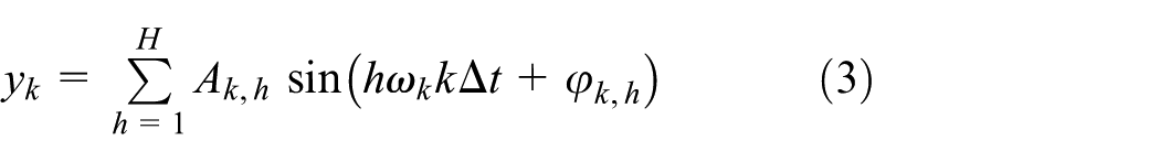
where
In order to estimate the state vector of the power system at the current time step k, given a group of measurements or observations

where the symbols are synonymous as above.
Having the measurement equations (2) and (3), process equation (1) and the state vector (4), we may establish the state transition matrix


What we should notice particularly is the dimensions of the above matrix and vectors. Since the dimension of state vector
Since the high-order harmonics are very small in real application, we only choose the first (fundamental), third, and fifth harmonics for simulation model in section “Simulation performance and harmonic parameter estimation.” Thus, the dimension of the filter is 7-by-7.
Proposed PF algorithm
This section is divided into two parts, which introduce the traditional PF algorithm and the proposed PF algorithm, respectively.
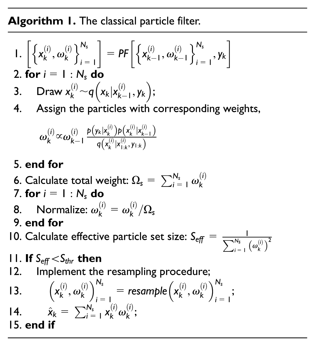
Classical PF algorithm
For non-linear and/or non-Gaussian systems, PF algorithms introduced by Gordon, which is also known as SIR, provide a practical and effective framework to perform filtering and smoothing for dynamic systems.
For state estimation problems, what we are actually concerned about is finding an appropriate estimator of
where

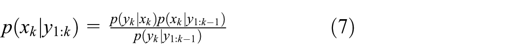
The probability density
However, the posterior PDF
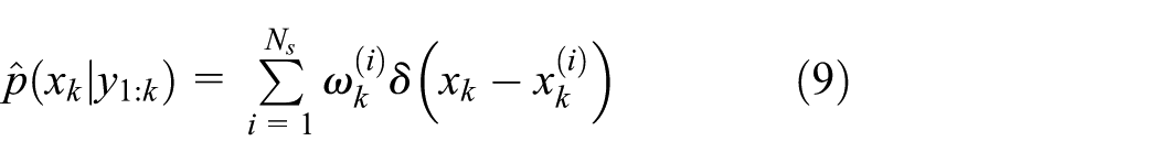
where
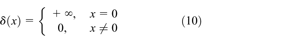
The idea of sequential importance sampling (SIS) is the basis of PF algorithm. We choose an importance distribution such that it factors similarly to the posterior density

making the weights satisfy

by considering equation (7), we have

and finally


It has been proven that using the SIS method above alone may lead to the particle degeneracy problem. That is to say, after a few iterations, most of the particle weights reduce close to 0, only one weight increases close to 1. This makes it a waste of computing resources and causes the algorithm become invalid. To avoid this phenomenon, the PF algorithm needs another step, referred to as resampling.
Normally, we use effective sample size

During each time step, the posterior distribution is resampled:
Proposed PF algorithm
The traditional PF algorithm introduced above has averted the particle degeneracy phenomenon by implementing resampling process. When implementing resampling, the idea of traditional PF algorithm is to draw samples (particles) from the PDF
Unlike other methods used by other researchers, we introduced several non-linear correlation coefficients into the algorithm. The advantage of this method is that it has good estimation accuracy without increasing the computational complexity of the algorithm (compared with the classical PF). In addition, most of the applicable systems of the algorithm are non-linear; therefore, the use of non-linear correlation coefficients can also avoid the inappropriateness of linear correlation coefficient in some non-linear cases.
Correlation coefficients
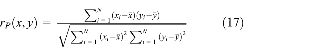
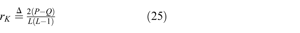
Correlation coefficient is defined and used quite frequently in statistics or mathematical analysis. It is a measure that determines the degree of two arrays’ variation tendency. There are several types of correlation coefficients that are perhaps the most widely used: Pearson’s linear correlation coefficient (Pearson’s r), Spearman’s rank-based coefficient (Spearman’s
As described above, correlation coefficients provide a measure of the strength and direction of the linear relationship between two time series. We will depict the definitions and structures of several different correlation coefficients below.
Define


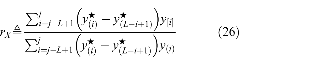
As proposed by Xu et al., 15 the order statistics correlation coefficient can be defined as

Correlation coefficients provide a measure of the strength and direction of the changing correlation relationship between two time series. Pearson’s r computes very fast; however, it may lead to a significant margin of error if non-Gaussian is involved in the model. The other three coefficients can be used under non-Gaussian condition with lower computation efficiency. Xu’s order statistic correlation coefficient provides the solution while offering a wider scope and more efficient application of correlation calculation.
Proposed PF algorithm
Zhou et al. 17 summarized kinds of methods for choosing the importance density directly or compositely and proposed a new way to choose the particles from importance density, which is based on Pearson correlation coefficient. Unlike the algorithm proposed by Zhou et al., the proposed algorithm in this article provides a new approach combining several different correlation coefficients with the resampling process to update particle weights. We also select other correlation coefficients instead of Pearson correlation coefficient due to its linear characteristic.
SIS method causes the degeneracy phenomenon and provides estimates whose variance increases exponentially with the discrete time index k. Resampling techniques are effective methods to solve this problem. Besides, applying the proposed methods in this article can also refresh the particles weights.
When implementing resampling, the idea of traditional PF algorithm is to draw samples (particles) from the PDF
During resampling process, particles chosen from the approximated posterior density according to the effective sample size
In HMM mathematic framework, since the independent observations of the true state
Step 1: Particles propagation. For
Step 2: Weights calculation. As illustrated in equation (14), particle weights can be recursively computed. Once we have the particle weights

Step 3: Initial resampling process. Compute the effective sample size
Step 4: Prepare two observation (measurement) arrays from the same time series.
Let k denote the discrete time index of the iterations,


Step 5: Calculate the correlation coefficient.
According to the definition of different rank correlation coefficients above, we get the corresponding equations as follows

where
Step 6: Adjust the parameter of corresponding weights.
When calculated the rank correlation coefficients of the two time series, we take the exponential function with an adjustable parameter
The proposed algorithm proceeds as follows. We can notice that the processes before resampling remain essentially unchanged. Hereafter, we abbreviate Spearman correlation coefficient resampling based particle filtering to SCCRPF, Kendall correlation coefficient resampling based particle filtering to KCCRPF, order statistic correlation coefficient resampling based particle filtering to OCCRPF, and collectively call them XCCRPF.

Justification
Smith and Gelfand
18
proved that if samples have upper boundary, the cumulative distribution function (CDF) of corresponding samples also has upper boundary under the customary bootstrap (particle filters). In this article, the screening procedure affected by the threshold
Suppose that samples
Density function
Simulation performance and harmonic parameter estimation
In this section, firstly we apply a one-dimensional model that has been analyzed in many publications before. Then we apply the proposed method to a given seven-dimensional state space model. The effectiveness of the proposed method is verified by comparing the parameter estimation results of different research methods.
One-dimensional model
The following example of simulation is well known and has been analyzed in many publications before. It is noteworthy that we set the process noise as a Gaussian mixture heavy-tailed distribution instead of a common Gaussian distribution in order to test the effectiveness and reliability of the proposed method more rigorously


where

where
The simulation algorithm was coded using MATLAB, and the program was performed on an Inter Core i5-4570 PC of 3.2 GHz and 4 GB memory. In order to assess the performance of different algorithms, we can use the root-mean-square error (RMSE) as criterion. The RMSE is given by

where
Simulation results of different algorithms.
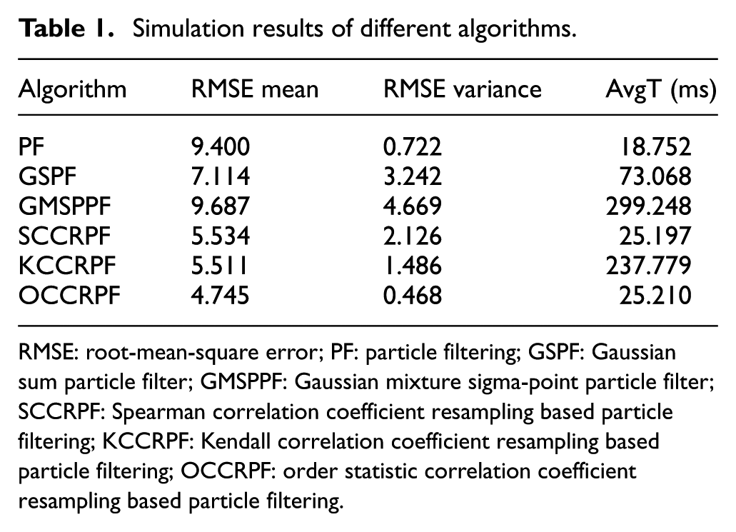
RMSE: root-mean-square error; PF: particle filtering; GSPF: Gaussian sum particle filter; GMSPPF: Gaussian mixture sigma-point particle filter; SCCRPF: Spearman correlation coefficient resampling based particle filtering; KCCRPF: Kendall correlation coefficient resampling based particle filtering; OCCRPF: order statistic correlation coefficient resampling based particle filtering.
Figure 1 shows the state estimation results of different algorithms in one simulation experiment. Different algorithms are marked in several different colors for the sake of convenience as illustrated in the legend. RMSE values of 10 random simulation runs of different algorithms are plotted in Figure 2. It is shown that the performance of the proposed algorithms is better than the PF, GSPF, and GMSPPF algorithms, while the three proposed algorithms perform similarly. In Table 1, KCCRPF’s extra time consumption is due to the computational complexity of Kendall’s

State estimation results of different algorithms.

RMSE of different algorithms.
Seven-dimensional model
As the above-mentioned model established in section “Harmonic parameter model,” we consider establishing a concrete seven-dimensional model to estimate the harmonic parameters in power system. The simulation signal is set as follows

The state equation and observation equation in matrix are as follows


where
The initial state was set to

In practical harmonic control, odd harmonics appear more frequently than even harmonics. In a balanced three-phase system, even harmonics have been eliminated due to the symmetrical relationship, and only odd harmonics exist. Because of this, we only choose odd harmonics in the simulation. The process noise is

where
We introduced the EKF algorithm as a contrast to show the superiority of the proposed algorithm. The EKF applies the Kalman filter to non-linear systems by simply applying the first-order approximation of Taylor series of the non-linear models. We wanted to do this because the relative simplicity and practical efficacy had made the EKF one of the most widely used algorithms in multiple fields.
The simulation runs for 200 steps, and the results are shown in Figure 3. Observations
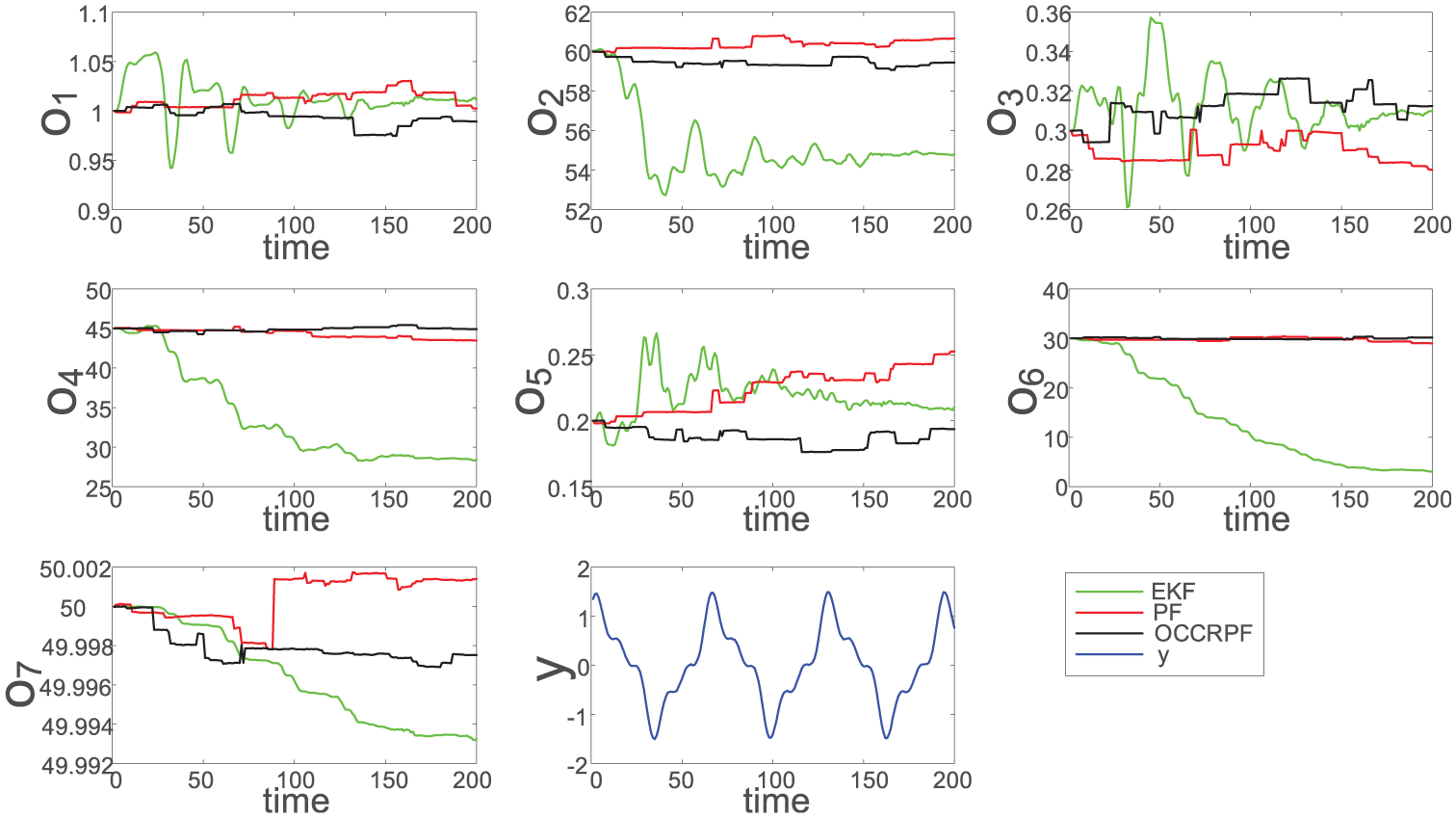
State estimation results of harmonic model.
As can be seen from Figure 3, the EKF algorithm tends to be stable after a period of oscillation, but its estimation value is biased and has a large error. Especially, for the estimation of phase angle, the deviation is large. The PF and OCCRPF algorithms perform better than the EKF algorithm. The estimation results of the amplitudes by PF and OCCRPF algorithms are similar to those by the EKF algorithm, while the fluctuation is smaller in the estimation process. For the estimation of phase angles, the PF and OCCRPF algorithms are obviously better than EKF. For the estimation of the utility frequency, the difference between the three algorithms is not significant, and the stability estimation values of the three algorithms are within fractions of the actual value.
Talking to the estimation effect of one single algorithm, EKF is the worst, especially for the estimation of the phase angle. The reason can be seen from the state transition matrix equation (5) and the measurement matrix equation (6). The estimations of odd terms of the state vector maintain linear variation, while the estimations of even terms of the state vector are originally from the function of sinusoid, which exhibit its non-linear characteristics. It is also well known that EKF can only give biased estimation for non-linear systems. This leads to errors of the estimation results of EKF. There is another reason why the accuracy of performance of the EKF algorithm was poor in the simulation. The issue is the parameter setting of process noise. We set the same noise parameters for the amplitude and phase variables. The phase vector has a non-linear calculation process of trigonometric function, which enlarges the deviation between the estimated and true value, thus further enlarging the phase error. As mentioned previously, there are no such problems for PF and OCCRPF algorithms.
Conclusion
In this article, a new particle filter algorithm combing with different rank correlation coefficients is proposed. Different rank correlation coefficients are introduced to measure the variation tendency between the particles and the state, and therefore obtain the particle weights. Compared with the PF, GSPF, and GMSPPF, the proposed method has better performance of estimation accuracy, and the computation time consumes about the same. Moreover, the computational complexity of the proposed algorithm is lower than GSPF and GMSPPF, which can be reflected by time consumption in Gaussian mixture noise.
A practical harmonic model of power signal is also simulated in this article. The simulation compared the EKF, PF, and OCCRPF algorithms. Because of non-linearity, EKF made biased estimates of state variables, especially for the phase variables. When it comes to PF and OCCRPF, the estimation of phase variables is much better than PF. Error analysis and simulation results show that PF and OCCRPF are superior to EKF for non-linear systems.
The algorithm proposed in this article leads to at least two interesting directions for continued research. First, because the computation accuracy of KCCRPF is well but causes high time consumption, new approach will be analyzed to reduce the time consumption of calculating Kendall’s
Footnotes
Handling Editor: Daming Zhou
Declaration of conflicting interests
The author(s) declared no potential conflicts of interest with respect to the research, authorship, and/or publication of this article.
Funding
The author(s) disclosed receipt of the following financial support for the research, authorship, and/or publication of this article: This work has been supported by the National Natural Science Foundation of China (no. 51277080).