New gradient methods for sensor selection problems

Abstract

In this article, we consider the sensor selection problem of choosing $T$ sensors from a set of $m$ possible sensor measurements. The sensor selection problem is a combinational optimization problem. Evaluating the performance for each possible combination is impractical unless $m$ and $T$ are small. We relax the original selection problem to be a convex optimization problem and describe a projected gradient method with Barzilai–Borwein step size to solve the proposed relaxed problem. Numerical results demonstrate that the proposed algorithm converges faster than some classical algorithms. The solution obtained by the proposed algorithm is closer to the truth.

Introduction

With the wide application of sensor networks in many fields (robotics, target tracking, medical health monitoring, traffic control, etc.),^1–8 all kinds of technologies related to sensor networks have been highly concerned by researchers. When sensor networks are used for target tracking, sensors communicate and process information for tracking targets. Due to the limited energy of sensors themselves, unnecessary energy consumption caused by communication and information processing will lead to premature paralysis of sensor networks. At the same time, excessive use of a few sensor nodes to track the target leads to the exposure of the node, which is attacked by the enemy (such as the radar sensor network). Therefore, in order to reduce the energy consumption of sensor nodes and increase the concealment, it is necessary to study the sensor selection problems.

Sensor selection problems study how to select $T$ sensors from $m$ sensors, which makes the fusion center based on these $m$ sensors observation data estimates the most accurate state of the target system. There are $c_m^T$ possible combinations when we choose $T$ sensors from $m$ sensors. When $m$ and $T$ are small, the optimal solution can be obtained by the exhaustive search, but the time spent on the optimal solution when both are larger is unbearable by the current computer. For example, when $m=100$ and $T=25$ , the search times will be $c_{100}^{25}\approx {10}^{23}$ , which requires very high computational efficiency.

For the objective of estimating the state of a given system, there has been growing literature in the past few years that study how to dynamically select sensors at run time to minimize certain metrics of the error covariance. The information theoretic framework and Bayesian framework for sensor selection problems are formulated in previous works.^9–14 In Chepuri and Leus’ ¹⁵ work, the sensor selection problem is formulated to nonlinear measurement models using the Cramer–Rao bound as the sensor selection criterion. Global optimization techniques, such as branch and bound,^16,17 are important approaches for solving the sensor selection problem exactly. Other approaches such as exploiting the submodularity of the objective function, heuristics based on genetic algorithms,^18–20 and greedy algorithms ²¹ are proposed to solve the sensor selection problem approximately. In Patan, ²² the author studies the estimation of distributed system parameters through the sensor observation data. The goal is to use the fewest sensor nodes to obtain the most accurate estimate, and the authors establish a multi-objective optimization model and solve the model with sequential quadratic programming based on branch and bound strategy. Joshi and Boyd ²³ propose a heuristic algorithm based on convex optimization and give the optimal sensor selection subset and optimality of upper bound. Numerical results show that the gap between the obtained solution and the optimal solution is small in most cases.

In this article, our goal is to minimize the volume of the associated confidence ellipsoid, which equals to the determinant of the estimation error covariance matrix. We propose to use projected gradient method, which requires less memory and is practical, for the relax sensor selection problem. We formulate the projection subproblem into searching the root of the piecewise continuous function. What is more, we introduce the Barzilai–Borwein (BB)^24,25 step size to avoid line search in traditional gradient method.

The article is organized as follows. In the next section, we introduce the sensor selection problem and give the corresponding optimization problem. The proposed algorithms are presented to solve the relax sensor selection problem in Section 3. Section 4 describes the compared results with traditional algorithms for sensor selection problem. Finally, the article is concluded in Section 5.

Sensor selection problem

Consider the problem of estimating a vector $x\in R^n$ from $m$ linear measurements, corrupted by additive noise

$$y_i=a_i^{T}x+{\eta }_i,i=1,2,\dots ,m$$

(1)

where $y_i\in R$ , $a_i\in R^n$ is the observation from the $i$ th sensor, ${\eta }_i$ represents the zero-mean Gaussian noise with variance ${\sigma }^2$ , and $x\in R^n$ is a vector of parameters to estimate. The maximum-likelihood estimate probability (MLP) estimate of $x$ is given by

$$\hat{x}={\left(\sum _{i=1}^m{a}_i{a}_i^T\right)}^{-1}\sum _{i=1}^m{y}_i{a}_i$$

(2)

The estimation error $x-\hat{x}$ has zero mean and covariance

$$\Sigma ={\sigma }^2{\left(\sum _{i=1}^m{a}_i{a}_i^T\right)}^{-1}$$

(3)

The $\eta -\mathrm{confidence}$ ellipsoid for $x-\hat{x}$ , which is the minimum volume ellipsoid that contains $x-\hat{x}$ with probability $\eta$ , is given by

$${ϵ}_{\alpha }=\{z|z^T{\Sigma }^{-1}z\le \alpha \}$$

(4)

where $\alpha =F_{{\chi }_n^2}^{-1}(\eta )$ , and $F_{{\chi }_n^2}(\eta )$ is the cumulative distribution function of a $\chi -$ squared random variable with $n$ degrees of freedom. A scalar measure of the quality of estimation is the volume of the $\eta -\mathrm{confidence}$ ellipsoid

$$\mathrm{vol}({ϵ}_{\alpha })=\frac{{(\alpha \pi )}^{n/2}}{\mathrm{\Gamma }\left(\frac{n}{2n+1}\right)}\det {\Sigma }^{1/2}$$

(5)

where $\mathrm{\Gamma }$ is the gamma function. Another scalar measure of uncertainty that has the same units as the entries in the parameter $x$ is the mean radius, defined as the geometric mean of the lengths of the semi-axes of the $\eta -\mathrm{confidence}$ ellipsoid

$$\rho ({ϵ}_{\alpha })=\sqrt{\alpha }(\det \Sigma {)}^{1/2n}$$

(6)

We will be interested in volume ratios, and so it is convenient to work with the log of the volume

$$\log \mathrm{vol}({ϵ}_{\alpha })=\beta -\left(\frac{1}{2}\right)\log \det \left(\sum _{i=1}^m{\alpha }_i{\alpha }_i^T\right)$$

(7)

where $\beta$ is a constant that depends only on $\sigma$ , $n$ , and $n$ . The log volume of the confidence ellipsoid, given in equation (7), gives a quantitative measurement of how informative the collection of $m$ measurement is.

The task of sensor selection is selecting a subset of $T\ge n$ sensors from the set of $m$ sensors such that the estimation error is minimized. We introduce a binary vector to represent the selection scheme

$$w=(w_1,w_2,\dots ,w_m{)}^T,w_i\in \{0,1\}$$

(8)

where $w_i$ indicates whether or not the $i$ th sensor is selected. The corresponding sensor selection problem is formulated as the following optimization

$$\begin{array}{cc}\min \hfill & \{f(w)=-\log \det \left(\sum _{i=1}^m{w}_i{a}_i{a}_i^T\right)\}\hfill \\ \multicolumn{1}{c}{\mathrm{s}.\mathrm{t}.}& w_i\in \{0,1\},i=1,2,\dots ,m\hfill \\ \multicolumn{1}{c}{}& 1^{T}w=T\hfill \end{array}$$

(9)

where the vector $1$ is the vector with all entries one. We note that the problem in equation (9) is a Boolean-convex problem, since $f(w)$ is convex for $w_i\ge 0$ , the first constraint is linear, and the selection vector $w$ is restricted to be $0$ or $1$ .

The proposed method

The Boolean constraints in problem of equation (9) make it difficult to solve directly. By relaxing each Boolean variable $w_i\in \{0,1\}$ to its convex hull $w_i\in [0,1]$ , we obtain the following convex relaxation problem

$$\begin{array}{cc}\min \hfill & \{f(w)=-\log \det \left(\sum _{i=1}^m{w}_i{a}_i{a}_i^T\right)\}\hfill \\ \multicolumn{1}{c}{\mathrm{s}.\mathrm{t}.}& 0\le w_i\le 1,i=1,2,\dots ,m\hfill \\ \multicolumn{1}{c}{}& 1^{T}w=T\hfill \end{array}$$

(10)

where $z\in R^m$ is the variable.

Joshi and Boyd ²³ propose a Newton’s method for solving the approximate relaxed sensor selection problem of equation (9), which is

$$\begin{array}{c}\min \{F(w)=-\log \det \left(\sum _{i=1}^m{w}_i{a}_i{a}_i^T\right)\hfill \\ \multicolumn{1}{c}{-\gamma \sum _{i=1}^m(\log (w_i)+\log (1-w_i))\}}\\ \multicolumn{1}{c}{\mathrm{s}.\mathrm{t}.1^{T}w=T}\end{array}$$

(11)

where $\gamma$ is a positive parameter that controls the quality of approximation.

Let ⊗ denote the Hadamard product and $A$ be the measurement matrix

$$A=\left[\begin{array}{c}{a}_1^T\hfill \\ \multicolumn{1}{c}{a_2^T}\\ \multicolumn{1}{c}{⋮}\\ \multicolumn{1}{c}{a_m^T}\end{array}\right]$$

(12)

The Hessian matrix of $F(w)$ in equation (11) is

$$\begin{array}{c}\multicolumn{1}{c}{{\nabla }^{2}F(w)=(\mathrm{AW}{A}^T)\otimes (\mathrm{AW}{A}^T)+\gamma \mathrm{diag}}\\ \multicolumn{1}{c}{(\frac{1}{z_1^2}+\frac{1}{{(1-z_1)}^2},\dots ,\frac{1}{z_m^2}+\frac{1}{{(1-z_m)}^2})}\end{array}$$

(13)

where

$$W={\left(\sum _{i=1}^m{w}_i{a}_i{a}_i^T\right)}^{-1}$$

The dominated cost of computing the Cholesky factorization in Newton step is $O(m^3)$ . When the number of $m$ is small, Newton’s method has high efficiency in solving equation (11). With $m$ increases, the memory requirement and computational cost become critical in Newton’s method. It brings about numerical difficulty when computing the inverse of ${\nabla }^{2}f(w)$ when $m$ is large.

In this article, we propose a projected gradient method for solving equation (10) directly. Let $\mathrm{\Omega }$ be the feasible region of equation (10). At iteration $k$ , projected gradient method computes the next point $w^{k+1}$ as follows

$$w^{k+1}=P_{\mathrm{\Omega }}(v^k)$$

(14)

where $v^k=w^k-{\beta }^k\nabla f(w^k)$ and

$$\nabla f(w^k)=\left[\begin{array}{c}{a}_1^{T}W{a}_1\hfill \\ \multicolumn{1}{c}{a_2^{T}W{a}_2}\\ \multicolumn{1}{c}{⋮}\\ \multicolumn{1}{c}{a_m^{T}W{a}_m}\end{array}\right]$$

(15)

$P_{\mathrm{\Omega }}(v^k)$ is the projection of $v^k$ onto the feasible region, that is, $w^{k+1}$ is the solution to

$$\begin{array}{cc}\min \hfill & \{q(w)=\frac{1}{2}\parallel w-v^k{\parallel }_2^2\}\hfill \\ \multicolumn{1}{c}{\mathrm{s}.\mathrm{t}.}& 0\le w_i\le 1,i=1,2,\dots ,m\hfill \\ \multicolumn{1}{c}{}& 1^{T}w=T\hfill \end{array}$$

(16)

Let ${\varphi }_{\lambda }(w)$ be the Lagrangian penalty function of $q(w)$ , that is

$${\varphi }_{\lambda }(w)=q(w)-\lambda (1^{T}w-T)$$

(17)

where $\lambda$ is a penalty parameter. For any given $\lambda$ , the solution to the following box-constrained problem

$$\begin{array}{cc}\underset{w}{\min }\hfill & {\varphi }_{\lambda }(w)\hfill \\ \multicolumn{1}{c}{\mathrm{s}.\mathrm{t}.}& 0\le w_i\le 1,i=1,2,\dots ,m\hfill \end{array}$$

(18)

is

$$w(\lambda )=\mathrm{mid}(0,h(\lambda ),1)$$

(19)

where $h(\lambda )=v^k+\lambda 1$ , and $\mathrm{mid}(.,.,)$ supplies the median of three componentwise arguments.

According to the Karush–Kuhn–Tucker (KKT) conditions for equation (16), $w({\lambda }^{*})$ is the KKT point of equation (16) if ${\lambda }^{*}$ makes

$$r({\lambda }^{*})=1^{T}w({\lambda }^{*})-T=0$$

Since $q(w)$ is strongly convex, $w({\lambda }^{*})$ is the unique global minimizer. Now, we consider how to find the root of $r({\lambda }^{*})$ . When $w(\lambda )=h(\lambda )$

$$r(\lambda )=\sum _{i=1}{v}_i^k+m\lambda -T$$

is a monotone increasing function. Thus, $r({\lambda }^{*})$ is either constant or a monotonically increasing function of $\lambda$ . A feasible approach for the solution of $r({\lambda }^{*})=0$ is the half-interval search (Algorithm 1). Once ${\lambda }^{*}$ is located, the next point $w^{k+1}=\mathrm{mid}(0,h({\lambda }^{*}),1)$ .

Algorithm 1. Half-interval Search

1: Initial interval $[{\lambda }_l^1,{\lambda }_r],r({\lambda }_l^1)\le 0,r({\lambda }_l^r)\ge 0,k=1$ . 2: while $|{\lambda }_l^k-{\lambda }_r^k|>ϵ$ do 3:   ${\lambda }^k=\frac{1}{2}({\lambda }_l^k+{\lambda }_r^k)$ 4:  if $r({\lambda }^k)\ge 0$ then 5:    ${\lambda }_r^{k+1}={\lambda }^k$ 6:    ${\lambda }_l^{k+1}={\lambda }_l^k$ 7:  else 8:    ${\lambda }_l^{k+1}={\lambda }^k$ 9:    ${\lambda }_r^{k+1}={\lambda }_r^k$ 10:  end if 11:   $k=k+1$ 12: end while 13: ${\lambda }^{*}=\frac{1}{2}({\lambda }_l^k+{\lambda }_r^k)$

It is well known that gradient method is often the only practical option in many engineering problems, but it has been observed that the sequence $w^k$ converges quite slowly to a solution. Nesterov ²⁶ proposes to use multistep version of an accelerated gradient method for constrained optimization problems with an attractive iteration complexity of $O(1/\sqrt{ϵ})$ for achieving $ϵ-$ optimality. Let $L$ be the lipschitz constant ²⁶ of $\nabla f(w)$ , Algorithm 2 is the framework of Nesterov algorithm for solving equation (10).

Algorithm 2. Nesterov Algorithm
1: Choose $z^1=w^0\in R^m$ , set $k=1$ , $t_1=1$ . 2: while not convergent do 3:   $w^k=P_{\mathrm{\Omega }}(z^k-\frac{1}{L}\nabla f(z^k))$ 4:   $t_{k+1}=\frac{1+\sqrt{1+4t_k^2}}{2}$ 5:   $z^{k+1}=w^k+\frac{t_k-1}{t_{k+1}}(w^k-w^{k-1})$ 6:   $k=k+1$ 7: end while

Algorithm 2 is feasible if lipschitz constant $L$ is known. In fact, global convergence can be guaranteed if $L$ satisfies

$$f(z^k+d^k)\le f(z^k)+\nabla f(z^k{)}^T{d}^k+\frac{L}{2}{d^k}^T{d}^k$$

(20)

In Amir and Marc’s ²⁷ work, $L$ is estimated with backtracking. Let $L_0>0$ and $\eta >1$ , then $L={\eta }^t{L}_0$ , where $t$ is the smallest non-negative integer making equation (20) hold and $d^k=P_{\mathrm{\Omega }}(z^k-(1/{\eta }^t{L}_0)\nabla f(z^k))-z^k$ . Backtracking method will cost heavy computational efforts since function value and projection $P_{\mathrm{\Omega }}(.)$ needs to be calculated a lot of times.

In this article, we introduce BB step size as ${\beta }^k$ for equation (10). Let the vectors $s^k=w^{k+1}-w^k$ and $y^k=\nabla f(w^{k+1})-\nabla f(w^{k+1})$ , the BB formula can be obtained by solving the following problems

$$\parallel \frac{1}{{\beta }^{k+1}}{s}^k-y^k{\parallel }_2^2$$

(21)

or

$$\parallel s^k-{\beta }^{k+1}{y}^k{\parallel }_2^2$$

(22)

The solutions for equations (21) and (22) are

$${\beta }^k=\frac{(s^k,y^k)}{(y^k,y^k)}$$

(23)

and

$${\beta }^k=\frac{(s^k,s^k)}{(s^k,y^k)}$$

(24)

The BB formula can be seen as an approximation of Quasi-Newton condition. Due to its simplicity, efficiency, and low memory requirements, BB formula has been used in many applications. There are some other spectral methods that alternate between equations (23) and (24). ${\beta }^k$ is updated with an average of the most recent $M\ge 1$ iterations information. Since the performance of these variants in our experiments is close to the standard formula for equations (23) and (24), we will use equations (23) and (24) as step size ${\beta }^k$ .

Since the solution $w_i^{*}$ for equation (10) can be interpreted as the probability of selecting sensor $i$ , we can use $w_i^{*}$ to generate the $k$ sensors. Let $w_{i_1}^{*},w_{i_2}^{*},\dots ,w_{i_m}^{*}$ denote the elements of $w^{*}$ rearranged in descending order. The selection is the indexes corresponding to the $k$ largest elements of $w^{*}$ , that is

$$C=\{i_1,i_2,\dots ,i_T\}$$

(25)

Let $f^{*}$ , $L$ , and $F^{*}$ be the optimal value of equations (9)–(11), respectively, then the associate objective value

$$U=-\log \det \left(\sum _{j=1}^T{a}_{i_j}{a}_{i_j}^T\right)$$

(26)

where U is an upper bound of $f^{*}$ . $L$ and $F^{*}-2m\gamma$ are a lower bound of $f^{*}$ .

Experimental results

In this section, we report the numerical results of the proposed projected gradient methods for sensor selection problems in this article. All tests are conducted on a Windows 10 with MATLAB 2014. For sensor selection problems, we set $m=200$ and $n=30$ . Linear measurements $a_i,i=1,2,\dots ,m$ are generated randomly by Gaussian function, that is, $a_i~N(0,1)$ . We compare our BB algorithm with Newton algorithm and Nesterov algorithm for sensor selection problems. We choose equation (24) as the step size in BB algorithm. Newton algorithm solves equation (11) with $\gamma =0.001$ , and Nesterov algorithm solves equation (10) with $\eta =0.5$ . We choose the best hyperparameters in Newton and Nesterov algorithms by grid search methods. The initial point $w^0=\frac{T}{m}(1,1,\dots ,1{)}^T$ .

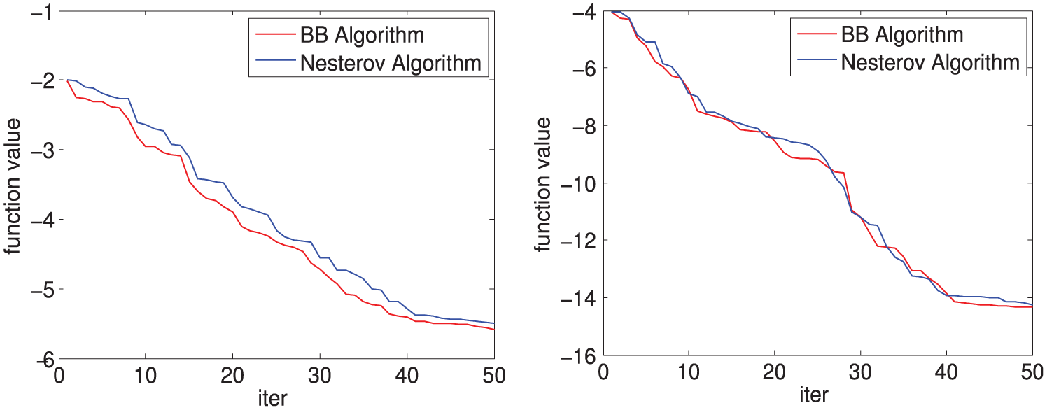
Figure 1 plots the function value of BB algorithm and Nesterov algorithm with $T=60$ and $T=80$ for equation (10), respectively. For $T=60$ , the proposed BB algorithm converges faster and gets lower function value than Nesterov algorithm. For $T=80$ , the proposed BB algorithm does not behave better than Nesterov algorithm in $40$ iterations. However, the proposed algorithm shows advantage in the last $10$ iterations.

Figure 1.

Function value with different $k$ in $50$ iterations: left: $T=60$ and right: $T=80$ .

Figure 2 shows the upper and lower bounds of the compared algorithms with $T\in [60,100]$ . From Figure 2, we can see that the bounds decrease as $T$ , since bigger $T$ means more observation $a_i{a}_i^T$ is accumulated in $f(w)$ . When $T=60$ , the upper bounds of BB algorithm is lower than the other two algorithms.

Figure 2.

Lower and upper bound of sensor selection problems: top left: Newton algorithm; top right: Nesterov algorithm; and bottom: BB algorithm.

Figure 3 plots the gaps between upper bounds and lower bounds as $T$ increases. On the whole, the gaps tend to decrease as $T$ increases. If the gaps is zero, the lower bound equals to upper bounds. In this case, the optimal indexes of sensor selection problem is equation (25). From Figure 3, we can see that the gaps of the proposed BB algorithm is lower than the other two algorithms, which means that the result of BB algorithm is closer to the optimal selection than the result of Nesterov algorithm and Newton algorithm.

Figure 3.

Gaps of the upper and lower bounds with Newton algorithm.

Conclusion and future work

We describe a projected gradient method with BB step size for the relax sensor selection problem. Numerical results also show that the new algorithm performs well on sensor selection problem. In this article, we consider only the volume of the confidence ellipsoid as the measure of estimation quality. Actually, there are other measures that can be used instead of this one, such as worst-case error variance. In the future, we will consider extending our BB algorithm for sensor selection problem based on other kinds of measures.