Sage Journals: Discover world-class research

Abstract

Internet of Medical Things is a smart provision of medical services to patients interacting with the doctors in harmony to uplift healthcare facilities. It enables the automated diagnosis of diseases for patients in remote areas. Alzheimer’s disease is one of the most chronic diseases and the main cause of dementia in human beings. Dementia affects the patient by a process of gradual degeneration of the human brain and results in an inability to perform daily routine tasks and actions. An automated system needs to be developed, to classify the subject with dementia and to determine the prodromal stage of dementia. Considering such requirement, a fully automated classification system is proposed. The proposed algorithm works on the hybrid feature vector combining the textural, statistical, and shape features extracted from three-dimensional views. The feature length is reduced using principal component analysis and relevant features are extracted for classification. The proposed algorithm is tested for both binary and multi-class problems. The method achieves the average precision of 99.2% and 99.02% for binary and multi-class classifications, respectively. The results outperform the existing methods. The algorithm showed accurate results with the average computational time of 0.05 s per magnetic resonance imaging scan.

Keywords

Alzheimer’s classification dementia principal component analysis brain magnetic resonance imaging segmentation Internet of Medical Things

Introduction

Alzheimer’s disease (AD) also simply referred to as Alzheimer’s is a severe neurological brain disorder. It is a degenerative process slowly damaging the brain cells. It initiates slowly and gradually grows worse by time. This results in the loss of the ability to perform day-to-day tasks along with short-term memory loss and behavioral issues.¹ According to a survey in 2015, almost 5.3 million people were suffering from Alzheimer’s in America. By 2050, the number is estimated to go up high to 16 million people.² It is a major cause of dementia and around 60%–70% of cases of dementia are suffering from Alzheimer’s.

In this age of science, still there is no proper treatment devised for Alzheimer’s;^3,4 however, if diagnosed early its progression can be determined. Magnetic resonance imaging (MRI) scans are used in the study of Alzheimer’s, the reason of which is the high contrast, good spatial resolution, and high accessibility.⁵ In various studies, feature extraction and classification are performed using the structural MRI. Features have been extracted from the region of interest (ROI), volume of interest (VOI),^6–8 gray matter (GM) voxels,⁹ and measurements of the hippocampus and morphometric methods.^10–12 Although various improvements have been recorded in early diagnosis of Alzheimer’s, yet the structural MRI has some room for further investigation and research.

AD is diagnosed using a careful medical assessment including patient history, mental state exam, and clinical dementia rating (CDR). Clinical data are accompanied by the MRI scan showing the structural and functional changes in the brain. The hippocampal region and cerebral cortex show a reduction in volume, whereas ventricles enlarge due to the AD. Such changes in the brain accompanied by the loss of memory and lack of planning, thinking, and judgment are significant signs to detect AD. These changes can be detected over MRI scans. However, for the development of a detection and classification system, clinical information supporting the medical imagery needs to be accompanied.

Today, in the era of modern technology, Internet of Things (IoT) solutions hold promising provision of smart healthcare services. To improve the healthcare facilities provided to the patients living in remote areas, smart computed tomography (CT) scanners are used to generate a vast flow of data for analysis and visualization purposes. This helps establish an interaction among the patients and doctors. The development of automated detection systems and the use of smart connected medical devices leads to an Internet of Medical Things (IoMT)-based diagnosis and decision system. The information provided by the smart medical devices such as CT scanners over the Internet is processed and the decision is made based on an automated detection system.

In this proposed methodology, an IoMT-based decision system for Alzheimer’s detection is proposed. The devices act as the individual nodes sending MRI scans covering the three views of the brain as sagittal, coronal, and axial over the cloud.

The images are then utilized by the decision system over the cloud to be processed. The images are scaled to a better contrast to achieve better segmentation results. The views are segmented using multi-level thresholding into regions of GM, white matter (WM), and cerebrospinal fluid (CSF). Textural, statistical, and shape features are extracted from the three-dimensional (3D) views of MRI scans. These features are combined to form a super-feature vector which is then reduced using the feature reduction technique. Classification is then performed over the features accompanied by CDR values as the ground data. Our proposed methodology contributes to the research area by

Proposing an IoMT-based architecture for the remote automated detection and decision of AD;

Developing an accurate Alzheimer’s detection system by incorporating the 3D views of MRI scans;

A hybrid feature-based classification model combining textural, statistical, and shape features;

Classifying the level of dementia as both binary class and multi-class problems handling the class imbalance problem.

The rest of the article is organized as follows: section “Related work” explains the existing work in this area, section “The proposed methodology” explains the methodology and section “Experimentation and results” shows all the experimental results followed by a conclusion.

Related work

The techniques developed for the detection of Alzheimer’s can be categorized into two groups based on the level of classification: binary and multi-class classifications; recent work done in both categories is discussed below.

Binary classification techniques

I Beheshti et al.¹ proposed a five-stage technique involving preprocessing, followed by image segmentation, resulting in individual segments of GM, WM, and CSF. Out of the segments, GM was utilized as ROIs that were used to build similarity matrices. Those matrices were then passed through the feature extraction stage resulting in statistical features. The statistical features combined with clinical data are then used to classify the test subjects into AD and normal. S Wang et al.⁴ proposed a method to classify the test subjects by estimating the 3D displacement field. The features were reduced using three feature selection techniques including Bhattacharyya distance, Student’s t-test, and Welch’s t-test. A support vector machine (SVM) classifier was trained over the feature vectors resulting in an overall accuracy of 93.05%.

A method was devised by I Beheshti et al.¹³ based on the significant GM volume reduction. Global and local shrinkage of GM was detected using voxel-based morphometry (VBM). The VOI was then segmented from the regions showing a significant contraction in the GM part of the brain. Features were then extracted from the VOIs, which are then optimized using genetic algorithm. The classification was performed using SVM giving an overall accuracy of 84.17%. A similar method was also utilized by Beheshti et al.¹⁴ where the regions depicting the significant volume reduction in GM were selected as VOIs. Voxel values from those regions were taken as raw features which were reduced later using various feature ranking techniques. The selected features based on their ranks were then classified using SVM giving an accuracy of 92.48%.

AK Ramaniharan et al.¹⁵ proposed a technique to analyze the changing shape of the corpus callosum segmenting T1-weighted MRI scans for Alzheimer’s detection. Laplace–Beltrami eigenvalue shape descriptor was used to extract the morphological features. The features were selected based on the ranking of information gain. The features were classified using SVM and K-nearest neighbor (KNN). KNN outperformed SVM giving a maximum accuracy of 93.37% with SVM achieving 91.67%.

A feature extraction framework was proposed by R Guerrero et al.¹⁶ based on the significant intersubject variability. A sparse regression model was used to derive the ROIs which were sampled for variable selection. The classification was performed giving an overall accuracy of 71%. A sulcal medial surface–based feature model was proposed by M Plocharski and Østergaard¹⁷ which were used to classify Alzheimer’s patients against cognitively normal (CN) subjects. The features were extracted from the distinct patient and were classified with an accuracy of 87.9%. Local features were extracted by O Ben Ahmed et al.¹⁸ from the region of the hippocampus and posterior cingulate using circular harmonic functions (CHFs). The classification was performed over the local features giving an accuracy of 62.07%.

For better classification results, deep learning algorithm was presented by S Sarraf et al.¹⁹ using convolutional neural networks (CNNs) along with auto-encoders. The technique provided promising results showing an overall classification accuracy of 98.4%.

Multi-class classification techniques

L Sørensen et al.²⁰ utilized features like cortical thickness, hippocampus texture, and shape. They combined these with the data from the MRI scans and a hybrid feature was proposed. The features were extracted from the Alzheimer’s Disease Neuroimaging Initiative (ADNI) database (http://adni.loni.usc.edu/) and trained over the linear discriminant analysis (LDA) classification algorithm. The technique showed an overall accuracy of 62.7% over the multi-class classification problem, classifying the subjects into healthy normal, mild cognitive impairment (MCI), and Alzheimer’s diseased. A multi-class classification technique is proposed in Altaf et al.²¹ using the combined features of the segmented images of GM, WM, and CHF. From these segments, textural and statistical features are extracted which are then used to classify the subject as an AD, MCI, and normal. The technique showed an overall accuracy of 79.8%. The algorithm was tested over the ADNI database.

In the previous techniques, binary and multi-class classifications of Alzheimer’s have been utilized. The focus in most of the methods was primarily on the binary classification of AD and MCI against the CN subjects. No technique in the literature was able to classify the subjects into multiple classes accurately. With such eminent research gap in this area, an accurate automated multi-class classification approach is proposed. Incorporating the selected features from the 3D views of the brain MRI leads to a significant improvement in Alzheimer’s detection and multi-class classification.

The proposed methodology

Our proposed method is a multi-staged classification algorithm that can take raw images as input from multiple smart CT scanners deployed over the network and automatically classify them as having AD or not. The possible IoMT-based architecture is shown in Figure 1. The illustration of the proposed methodology is shown in Figure 2. The pseudocode of the proposed system is given in Algorithm 1.

Figure 1.

IoMT-based architecture.

Figure 2.

The proposed methodology.

Algorithm 1. Alzheimer’s disease classification (which takes MRI scan as an input, performs segmentation feature extraction, and classifies the test images).
Input: gray-scale image of the brain MRI scan; verdict from the medical expert
Output: classification result; prediction of level of dementia
1: procedure LinearContrastStretching(img, img(i, j), maxlevel)
2: a = max(img)
3: b = min(img)
4: im_cs(i, j) = maxlevel((img(i, j*) – b)/(a – b))
5: returnim_cs(i, j)
6: end procedure
7: procedure MultilevelThresholding(img_cs, K)
8: (t₀, t₁, t₂, …, t_k_– 2) = thresholds (img, K)
9: N = f₀ + f₁ + f₂, …, f_L_– 1
10: fori = 1, L – 1
11: prob(i) = f(i)/N
12: end for
13: fori ∈ C(k)
14: cprob(k) = sum(prob(i))
15: end for
16: fori ∈ C(k)
17: m(k) = sum(i(prob(i)/cprob*(k)))
18: end for
19: fork = 0, K – 1
20: M = sum(m(k)*cprob(k))
21: end for
22: fork = 0, K – 1
23: Var = sum((cprob(k)*m(k))² – M²)
24: end for
25: return (max(Var(t₀, t₁, t₂, …, t_k*_– 2)))
26: end procedure
27: procedure FeatureExtraction(img_thresh)
28: (s₁, s₂, s₃, …, s_n) = Statisticalfeatures(img_thresh)
29: (t₁, t₂, t₃, …, t_n) = Texturalfeatures(img_thresh)
30: (sp₁, sp₂, sp₃, …, sp_n) = Shapefeatures(img_thresh)
31: return ((s₁, s₂, …, s_n),(t₁, t₂,…, t_n),(sp₁, sp₂, …, sp_n))
32: end procedure
33: procedure Featurereduction((s₁, s₂, …, s_n), (t₁, t₂, …, t_n), (sp₁, sp₂, …, sp_n))
34: reducedfeatures = PCA((s₁, s₂, …, s_n), (t₁, t₂, …, t_n), (sp₁, sp₂, …, sp_n))
35: return(reducedfeatures)
36: end procedure
37: procedure Classification((f₁, f₂, f₃, …, f_n), labels)
38: Model = training((f₁, f₂, f₃, …, f_n), groundlabels)
39: Predictedlabels = testing(Model, (f₁, f₂, f₃, …, f_n))
40: Accuracy = Confusionmat(Predicedlabels, groundlabels)
41: Classificationmap = map(Predicedlabels)
42: return Classificationmap
43: end procedure

The architecture is based on multiple patients at multiple hospitals under smart CT scanners. These scanners can be connected over the network (in this case Internet) each acting as an individual node. The nodes transfer the sensed data over the cloud which can then be processed by the processing unit. The processing unit classifies and decides the sensed output based on our proposed algorithm.

The proposed multi-staged algorithm used to process the collected scans over the IoMT-based architecture is elaborated in Figure 2 and is discussed in detail in the sections below.

Image preprocessing

Non-linearity in light intensity affects the performance of the medical image processing techniques. It is mainly introduced by the wrong set of lens aperture of medical imaging devices. Such images are then preprocessed using the image enhancement techniques.²² Contrast stretching is one of the basic techniques of image enhancement through which the intensity range of an image is normalized. There are many methods to extend the dynamic range of the image. However, linear stretching is a robust and efficient way to do it.

Linear contrast stretching

It is the linear enhancement of the dynamic range of gray levels. The range of the pixel values from minimum to maximum is stretched linearly so that the pixels at the lower levels are given a slightly higher value. This results in the transformation of dark pixels into brighter ones. This is a pixel-based operation where each input pixel is given an output value based on a transfer function. If x is the pixel value of the input image im, then the transformed pixel value y of the output image im′ is mapped by a linear transfer function given in equation (1)

y = c (\frac{x - b}{a - b})

(1)

where c is the maximum gray-level intensity of the output image; a and b are the maximum and minimum gray-level pixel values of the input image, respectively.²³ In our dataset, on average, pixels fall in the range of 0–226. In order to enhance the contrast of the images, linear contrast stretching is applied resulting in the curve map from input x to output y.

Image segmentation

In order to extract each of the brain components, their corresponding gray-level intensities are segmented as a group of similar intensities using multi-thresholding. For bilevel thresholding, Otsu’s method is very popular among the image segmentation techniques. It works on maximizing the interclass variance and finding the optimum value for that. Otsu’s method can be easily extended to the multi-level thresholding by selecting a global threshold value increasing the separability of clusters.²⁴ For an image represented in a total of L gray levels (0, …, L – 1), the number of pixels at each level is represented by f_i. The total number of pixels in the image will be given as $N = f_{0} + f_{1} + \dots + f_{L - 1}$ . The occurrence probability of each pixel i will be given in equation (2)

p_{i} = \frac{f_{i}}{N}, p_{i} ⩾ 0

(2)

If the image is to be segmented into K clusters using K – 1 thresholds (t₀, t₁, …, t_k_– 2) must be selected. The cumulative probability $ω_{k}$ and mean gray-level µ_k for each cluster C_k are computed as given in equations (3) and (4), respectively

ω_{k} = \sum_{i \in C_{k}} p_{i}

(3)

μ_{k} = \sum_{i \in C_{k}} i \frac{p_{i}}{ω_{k}}, k \in [1, \dots, K - 11, \dots, K - 1]

(4)

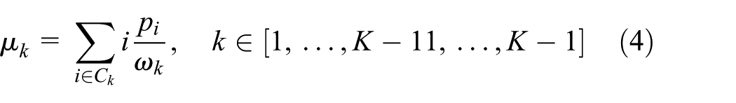
From the above extracted values, the average intensity value of the entire image µ_T and the interclass variance $σ_{B}^{2}$ are determined as given in equations (5) and (6), respectively

μ_{T} = \sum_{k = 0}^{K - 1} μ_{k} ω_{k}

(5)

σ_{B}^{2} = \sum_{k = 0}^{K - 1} ω_{k} μ_{k}^{2} - μ_{T}^{2}

(6)

The optimal thresholds are thus determined by maximizing the interclass variance as given in equation (7)

{t_{0}^{*}, t_{1}^{*}, \dots, t_{K - 2}^{*}} = \max {σ_{B}^{2} (t_{0}, t_{1}, \dots, t_{K - 2}}

(7)

Feature extraction

It is the calculation of distinctive characteristics of the segmented components to be classified accurately. The GM, WM, and CSF regions of the brain MRI scans after being extracted from the preprocessed input scan are represented by a set of features. Along with the progression of AD, the human brain tissue contracts causing the variation in the shape and texture along with the statistical characteristics of the human brain. These variations are characterized by extracting the respective features. These extracted features are statistical, textural, and morphological. Each of the feature extraction technique resulting in the calculation of the hybrid feature vector is discussed below. These techniques are grouped based on the type of features they are used to extract.

Statistical features

These features are derived from the histogram of gray-level intensities. The distribution and frequency of the gray-level intensities in the GM, WM, and CSF components of the brain MRI scans are used to calculate a set of statistical features. These features include mean, standard deviation, kurtosis, skewness, interquartile range (IQR), and geometric mean.²⁵ Each of the statistical features is briefly discussed below.

Mean

The average value calculated over the set of values of an image is the sum of the pixel values divided by the total number of pixels. It provides the mean value of a segment of our MRI scan images around which the rest of the pixels are positioned. For an image of size M × N, the mean of the image is calculated as given in equation (8)

Mean (μ) = \frac{\sum_{i = 1}^{M} \sum_{j = 1}^{N} im (i, j)}{M \times N}

(8)

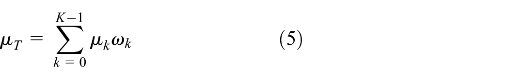
Standard deviation

It is a measure that is used to quantify the amount of variation or dispersion of a set of data values. A low standard deviation indicates that the data points tend to be close to the mean (also called the expected value) of the set, while a high standard deviation indicates that the data points are spread out over a wider range of values. It gives the range of values in which input segments of the MRI scan are presented. Standard deviation is calculated as given in equation (9)

Standard deviation (σ) = \sqrt{\frac{1}{M \times N} \sum_{i = 1}^{M} \sum_{j = 1}^{N} {(x_{i} - μ)}^{2}}

(9)

Kurtosis

Kurtosis represents the probability distribution of shape. It represents a function for tailedness of a probability distribution for a real-valued variable. It can be calculated as given in equation (10)

Kurtosis (k) = \frac{E {(im (i, j) - μ)}^{4}}{σ^{4}}

(10)

Skewness

It is a measure of the asymmetry of the probability distribution for a random variable and can be calculated as given in equation (11)

Skewness (s) = \frac{E {(im (i, j) - μ)}^{3}}{σ^{3}}

(11)

Geometric mean

The geometric mean is a type of mean or average, which indicates the central tendency or typical value of a set of numbers using the product of their values. The geometric mean is calculated as given in equation (12)

Geometric mean (G) = \sqrt[n]{im (i, j) \cdot im (i, j + 1) \cdot \dots}

(12)

IQR

It is a measure of variability within the data by dividing the data points into groups or quartiles. The value denotes the amount of dispersion of data. It is measured as the difference between the formed quartiles. The formula of IQR is given in equation (13) as

Interquartile range (IQR) = Q 3 - Q 1

(13)

Textural features

The texture is formed by the alternate position of the pixels in an image. It represents the spatial relationship between pixels at certain positions in an image. In order to capture the textural information of images, various textural feature extraction techniques are applied and their corresponding features are recorded. Each of the technique is briefly discussed below.

Gray-level co-occurrence matrix

It is listed as one of the earliest methods to extract textural features. Since its first utilization, it has been widely used in many textural analysis applications and as a feature extraction technique in the textural analysis domain.²⁶ Gray-level co-occurrence matrix (GLCM) works by forming a GLCM specifying the occurrence of gray levels at specific locations of the image. It calculates the frequency of pixels having value j forming a relationship with pixel p over a given area. In a gray-scale MRI, scan pixels are represented by the 8-bit intensity levels. These levels are varying over the special coordinates of an image. Such variation in the image forms a texture that can be calculated using GLCM. From the co-occurrence matrix, different features such as homogeneity, correlation, entropy, and contrast are extracted. Each of the distinctive features is discussed below.

Contrast

It is defined as the variation in the specific areas within the GLCM. The contrast is calculated as given in equation (14)

Contrast = \sum_{x, y} {| x - y |}^{2} \log P_{r, θ} (x, y)

(14)

where $P_{r, θ}$ is the co-occurrence matrix, (x, y) represents the transition of gray-level intensity from pixel x to pixel y, and r is the distance between the two pixels lying at an angle of $θ$ .

Correlation

It calculates the cumulative probability of a specified pixel pair co-occurring in the GLCM. It is given in equation (15) as

Correlation = \sum_{x, y} \frac{(x - μ_{1}) (y - μ_{2}) P_{r, θ} (x, y)}{σ_{1} σ_{2}}

(15)

where $μ_{1}$ and $μ_{2}$ are, respectively, the mean and standard deviation of the two images correlated.

Homogeneity

It measures the closeness of elements in the GLCM matrix to its diagonals which are measured as given in equation (16)

Homeogeneity = \sum_{x, y} \frac{P_{r, θ} (x, y)}{1 + {| x - y |}^{2}}

(16)

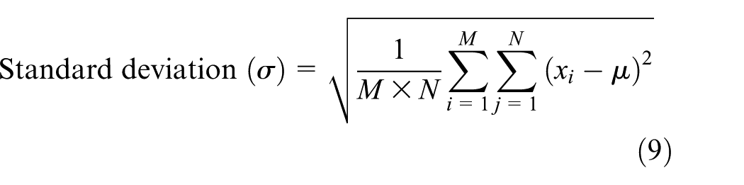
Entropy

It measures the amount of lack of order in an image. An image with a large entropy comprises a random texture. The relationship of entropy with the GLCM values is reversely proportional. It is calculated as given in equation (17)

Entropy = - \sum_{x, y} P_{r, θ} (x, y) \log P_{r, θ} (x, y)

(17)

Speeded-up robust features

Speeded-up robust feature (SURF) works on the approximation of the module of difference of Gaussian (DoG) with a box filter. The method performs Gaussian filtering over the individual boxes instead of filtering over the entire image.²⁷ This square-based convolution provides an efficient and robust technique. SURF determines the points of interest using the blob detector based on the Hessian matrix. The feature descriptors are acquired by calculating the wavelet responses around the neighborhood of the determined points. For each of the slice of MRI, scan SURF is calculated for the determined points.

Shape-based features—histogram of gradients

Features are the key descriptors used to identify ROI in an image. Objects are detected in an image using the key features required to represent them distinctively. The shape is an important feature to represent different regions within an image. Internal components of the brain show a distinctive variation in their texture along with the shape. The shape of these components varies with Alzheimer’s and other brain disorders in reference to a normal subject. Among the various shape-based feature extraction techniques, histogram of gradients (HoG) is used.

HoG determines the features of an image by calculating the frequency of variation in the pixels in a given region.²⁸ It utilizes the shape and edge information represented as a feature vector. The feature vector is composed of the shape information from different regions of the image. The histogram is calculated for angles with a difference of 45 degrees in all directions. A default window size of 8 × 8 was utilized to capture the required information over the image. The image given below is the HoG calculated over a 4 × 4 window size.

The class imbalance problem

The performance of the classification algorithms is severely affected by data quality, biased datasets, and the class imbalance problem. The class imbalance problem is mainly introduced when the examples of one of the classes are insufficiently presented. In simpler terms, the number of positive samples is much smaller than that of the negative ones. Many classification algorithms are accuracy driven and are trying to maximize accuracy. In class imbalance dataset, the classification accuracy highlights very little about the minority class. Since the datasets are influentially imbalanced, the lower recognition rate of the minority class is easily ignored resulting in high accuracies majorly depicting the detection rate of the majority class. It may lead to imprecise decisions causing erroneous judgments and an inaccurate detection system. The OASIS-1 dataset faces the class imbalance problem with a distinct variation in the ratio of the class-wise image. Among the 416 registered subjects, 305 MRI samples with available ground-truth classes were taken in which 205 images belonged to normal subjects, 70 belonged to very mildly demented subjects, 28 belonged to mildly demented, and only 2 belonged to moderately demented subjects. To rectify these problems, such classes should be properly handled and treated. Different techniques and remedies are used to handle the class imbalance problem. These methods are grouped into two categories. These categories are based on the data perspective and the algorithm perspective. Methods with the data perspective utilize standard data sampling techniques. These sampling techniques include oversampling and undersampling methods including random oversampling (ROS), random undersampling (RUS), and synthetic minority oversampling technique (SMOTE). In our proposed methodology, we have utilized SMOTE, as the undersampling methods reduce the number of samples and the random initialization in the oversampling reduces the diversity within the dataset.

SMOTE

It is an oversampling technique utilized to cope up with the class imbalance problem. It is a widely used technique balancing the distribution of samples from the minority class. SMOTE oversamples the instances of the minority class increasing its instances in the overall data samples. This oversampling is based on the KNN.²⁹ For the proposed algorithm, we have utilized the value of 5 for K. It works by taking a sample from the minority class and generating synthetic data in the direction of the nearest neighbors of that sample. The synthetic data are generated following a couple of key steps. The distance between the selected minority sample and the selected nearest neighbors is calculated at first and multiplied by a value between 0 and 1. Then, the resultant value from the first step is summed up with the selected sample. This results in the selection of a random point between the selected samples.

Feature selection

Feature selection is a process to select the most discriminative features and discard the redundant features. The main aim is to choose the optimal number of inputs by reducing the features that are having less significant predictive information. Feature selection is proven to enhance learning efficiency and predictive accuracy and to reduce complexity. As the dimensionality of a domain increases, the number of features also increases making it a likable situation to eliminate the irrelevant ones. A super-feature vector formed due to a combination of features of different types from the three views, which also resulted in the cumulative dimension. This posed a need for dimensionality reduction selecting appropriate features for robust functionality. However, the textural, statistical, and morphological characteristics play an important role in characterizing the MRI of a demented brain. Thus, each type of feature is significant in the super-feature vector. To maintain the significance of our features, among various feature extraction techniques, principal component analysis (PCA) has been utilized. PCA is a feature reduction technique and is mainly used due to the transformation of the existing features into principal components, that is, no existing feature is discarded. The principal components with high variances are selected and used as the distinctive feature set. PCA is a fast and robust technique reducing the dimensionality of the feature space with low computational cost.

PCA

PCA is one of the important feature selection techniques identifying the reasonable dimensions in the feature space. The identified dimensions are then selected solving the feature reduction problem.³⁰ PCA works by computing the principal components u_k as a linear combination of the reducible feature vector x_j. Principal components are calculated to examine the variance within the dataset. The first principal component is oriented in the direction of maximum variance with the following components in the direction of variance in decreasing order. Projection of features to the eigenvector w∼k is the most relevant combination having an association with the highest eigenvalue λ_k of the feature correlation matrix C. This provides the best information required. It results in the formation of the weighing coefficient w_jk for each component of the linear combination. In the end, the linear combination is represented by a projected vector u~ with k dimensions as given in equation (18)

u_{k} = \sum_{j} w_{j}^{k} x_{j}

(18)

Weighting depicts the contribution of the original reducible features to the linear combination. Feature reduction is performed using the above calculated coefficients.

Classification

Reduced 3D features from PCA are then fed into a classification stage to determine the level of dementia in the test subjects. For this purpose, we used different classification algorithms as naïve Bayesian, Bayesian networks (BayesNet), multi-layer perceptron (MLP), and random forest (RF). Working with each classification algorithm is briefly discussed below.

BayesNet

BayesNet is a strong representation of probabilistic functions and receives considerable attention in the machine learning and classification community. The prediction of a sample belonging to a class is purely based on the probability of the sample belonging to that class.³¹ Among the random variables, the BayesNet is a graphical model representing the probabilistic relationships. The finite set of variables is given as X = {X₁, X₂, …, X_n}, where each variable X_i may take value from a finite set represented by val(X_i).

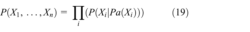
It is an annotated directed acyclic graph (DAG) G, encoding the joint probability over X. Random variables X₁, …, X_n represent the nodes of the graph. A directed relationship from node X_i to node X_j makes the former one a parent to the later node. Each node is represented with the conditional probability that shows P(X_i – Pa(X_i)), where Pa(X_i) represents the parent node of X_i in the DAG. The two (G, CPD) encode the joint probability P(X₁, …, X_n) given in equation (19)

P (X_{1}, \dots, X_{n}) = \underset{i}{Π} (P (X_{i} | Pa (X_{i})))

(19)

Naïve Bayesian classifier

Naïve Bayesian classifier uses the simple normal distribution for modeling numerical attributes. It is based on conditional probabilities. It uses the Bayes theorem that calculates the probability by counting the number of occurrences of values and the combination of values in the historical data. It determines the probability of an occurring event based on the prior probability of the events that have already occurred. The Bayes theorem is a relation of conditional and marginal probabilities of two random events. Let x = {x₁, x₂, x₃, …, x_d} be an instance of dimensions d having no class label. Let C = {C₁, C₂, …, C_K} be the set of class labels. P(C_k) is the prior probability of C_k. P(x|Ck) is the conditional probability of interpreting the evidence x if the hypothesis C_k is true. Posterior probability is calculated as given in equation (20)

P (C_{k} | x) = \frac{P (x | C_{k}) P (C_{k})}{\sum_{k'} P (x | C_{k'}) P (C_{k'})}

(20)

Naïve Bayes classifier works with the assumption that the value of a feature shares no relationship with any other as given in equation (21)

P (x | C_{k}) = Π_{j = 1}^{d} P (x^{j} | C_{k})

(21)

MLP

Artificial neural network (ANN) is a machine learning classification algorithm based on the inspiration from the human nervous system.³² ANN is the interconnection of artificially created groups called neurons. ANN is an adaptive classification algorithm adapting to the information passed both internally and externally through the network. Elements called as nodes are forming parallel connections resulting in an ANN network. During the training phase of the network, the weights of each node are adjusted based on the difference in the output and target class. The process is repeated iteratively until the difference between the output and target class becomes zero. ANN is a supervised learning classifier widely used due to its information storage ability. ANNs are further categorized into a single-layer and a multi-layer perceptron. A single-layer perceptron uses a single layer of weights connecting the output directly to the input. In MLP, the multiple layers are used between the input and output layers called as hidden layers. In this proposed methodology, an MLP-based ANN is used and back-propagation is utilized for training purposes.

RF

RF is very much popular among the classifiers due to its high performance compared to the others. It is based on an ensemble technique grouping many week classifiers like decision trees and classifies the instances by summation of their individual votes.³³ Its high performance is mainly due to utilizing the advantage of two classification techniques: bagging and random feature selection. Trees are generated utilizing the bootstrap samples from the training data. The top-down approach is followed favoring the diversity of the ensemble method. Prediction is made based on the majority vote. Each tree is designed using a subset of original features. Afterward, the classifier creating other trees at each node splits the features. Each tree is then built to its maximum extent. Classification is performed based on majority votes.

Experimentation and results

Dataset

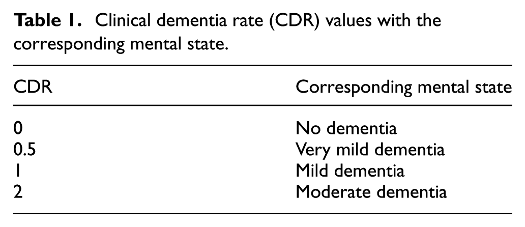
The dataset used for training of our system is collected from OASIS. The site offers a public data repository for research purposes. The dataset covers the cross-sectional brain MRI scans of various subjects from the age of 18 to 96. The images are covering images from the sagittal, coronal, and axial planes of the human brain. This provides a 3D view of the human brain MRI scan. To test the proposed algorithm, MRI scans from the smart CT scanners have been acquired which were deployed at multiple hospitals connected over the Internet. Each scanner acts as a node of IoMT architecture. The nodes transfer the data over the cloud which are processed further, and the decision is made. The images acquired are gray-scaled that cover subjects with no, very mild dementia, mild, or moderate dementia. The dataset is formed by taking 70% of images from the public dataset OASIS and 30% of images through smart CT scanners. Images are supported by the CDR from medical experts.³⁴ These CDR values along with their diagnosed condition are shown in Table 1.

Table 1.

Clinical dementia rate (CDR) values with the corresponding mental state.

CDR	Corresponding mental state
0	No dementia
0.5	Very mild dementia
1	Mild dementia
2	Moderate dementia

Accuracy assessment

In order to evaluate our classification system tested over the OASIS dataset, various accuracy assessment metrics were used. These metrics included precision, recall, F1-measure, and ROC.²⁹ Each of the metrics is briefly discussed here.

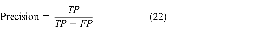
Precision is the effectiveness of the classification system. Through precision, we can evaluate the relevancy of the detection by the system. It is mathematically calculated in equation (22)

Precision = \frac{TP}{TP + FP}

(22)

Recall determines the probability of detection of a particular class. It gives the ability of a model to detect all relevant classes. Mathematically, it is given in equation (23) as

Recall = \frac{TP}{TP + FN}

(23)

In the above two equations, TP is the true positives that are true samples classified correctly by the system. Samples that have no disease are predicted to be healthy. FP is the false positives that are the samples predicted not to have the disease though in reality they do. FN is the false negative where the samples are predicted to have a disease; however, in ground data they do not. FN and FP show the misclassification of results.

F1-measure is the optimal combination of precision and recall. It is said to be the harmonic mean of precision and recall. Taking both accuracy metrics into account, the equation is given as

F 1 = 2 * \frac{Precison * Recall}{Precison + Recall}

(24)

Statistically, the receiver operating characteristic (ROC) curve is a graphical representation of diagnostic proficiency of the classification system. It is generated by plotting the true-positive rate (TPR) against the false-positive rate for varying threshold values.

Experimental setup

Cross-validation is used to evaluate the performance of classifiers. In this work, we have used k-fold cross-validation. In cross-validation, the dataset is equally divided into k folds and then each single fold is used for testing and the remaining folds are used for training. This process is iteratively run until all folds are used for testing and the average results are shown.

Results and discussion

Our proposed system was trained and tested over the images acquired from the OASIS database, but this trained system can be used to test the images acquired from smart CT scanner images for both binary and multi-class problems. Segmentation refers to the partitioning of an image into disjoint segments that share a uniform intensity and gray levels. WM, GM, and CSF are the components commonly used to represent brain tissue compartmental models.³⁵ These components are captured collectively in an MRI scan. The segmented components are shown in Figure 3. However, their varying intensities provide a room for segmenting each of the components separately.

Figure 3.

Linear contrast stretching for y = 1.128x.

Performance evaluation in terms of binary classification

In the binary class problem, the test subjects were classified as CN or AD. The subjects were having a different level of dementia based on their CDR values. In the binary class problem, subjects having very mild dementia, mild dementia, and moderate dementia were all categorized as Alzheimer’s. Classification results from different classifiers were then evaluated over the accuracy assessment metrics. Results from each of the classification algorithm are shown in Table 2. In a binary classification problem, RF outperformed the rest of the classification algorithms. The classification results are obtained over the publicly available dataset; however, the system gives equally accurate results for the images acquired over the IoMT architecture.

Table 2.

Accuracy metrics for binary classification.

S. No.	Classification algorithm	Precision	Recall	F1-measure
1	Bayes network	98.8	98.8	98.8
2	Naïve Bayesian	98.4	98.4	98.4
3	Multi-layer perceptron	97.7	97.6	97.6
4	Random forest	99.2	99.2	99.2

Performance evaluation in terms of multi-class classification

The multi-class classification has always been the major classification problem when it comes to AD. The level of dementia and mental state of a human mind are challenging to determine. A high accuracy was achieved in the classification of CN against the AD subjects. The subjects are classified based on the CDR values depicting subjects having no dementia, very mild dementia, mild dementia, and moderate dementia. The classification results for the multi-class problem were recorded, and it is observed that all the classification algorithms outperformed the results in the literature. The accuracy assessment of all the classifiers is given in Table 3.

Table 3.

Accuracy assessment metrics for multi-class classification.

S. No.	Classificationalgorithm	Precision	Recall	F1-measure
1	Bayes network	98.775	98.775	98.775
2	Naïve Bayesian	99.025	99.025	99.025
3	Multi-layer perceptron	97.075	96.8	96.8
4	Random forest	98.975	98.975	98.975

In the multi-class problem, among the four classification algorithms, naïve Bayesian showed an overall commendable performance. Each of the accuracy assessment metrics showed a high performance rate among the rest.

Comparative analysis of our proposed system with the use of K-means clustering

Among the various image segmentation techniques, K-means clustering is one of the most widely used algorithms in the field of image processing. The algorithm works on extracting pixels with similar intensity levels from the background in the form of non-overlapping groups.

The algorithm extracts the desired information by initializing the K centroids around which the clustering process takes place. The process repeats itself iteratively until the centroids converge to their final constant position. Utilization of K-means clustering in our algorithm produces almost equal segmentation results (Figure 4); however, the computational complexity increases, thus increasing the computational time. Our proposed system resulted in an average computational time of 0.05 s per image with the utilization of multi-level thresholding for segmentation (Figure 5). However, with the use of K-means clustering for segmentation, the algorithm almost doubled the computational time increasing the average time to 0.108 s.

Figure 4.

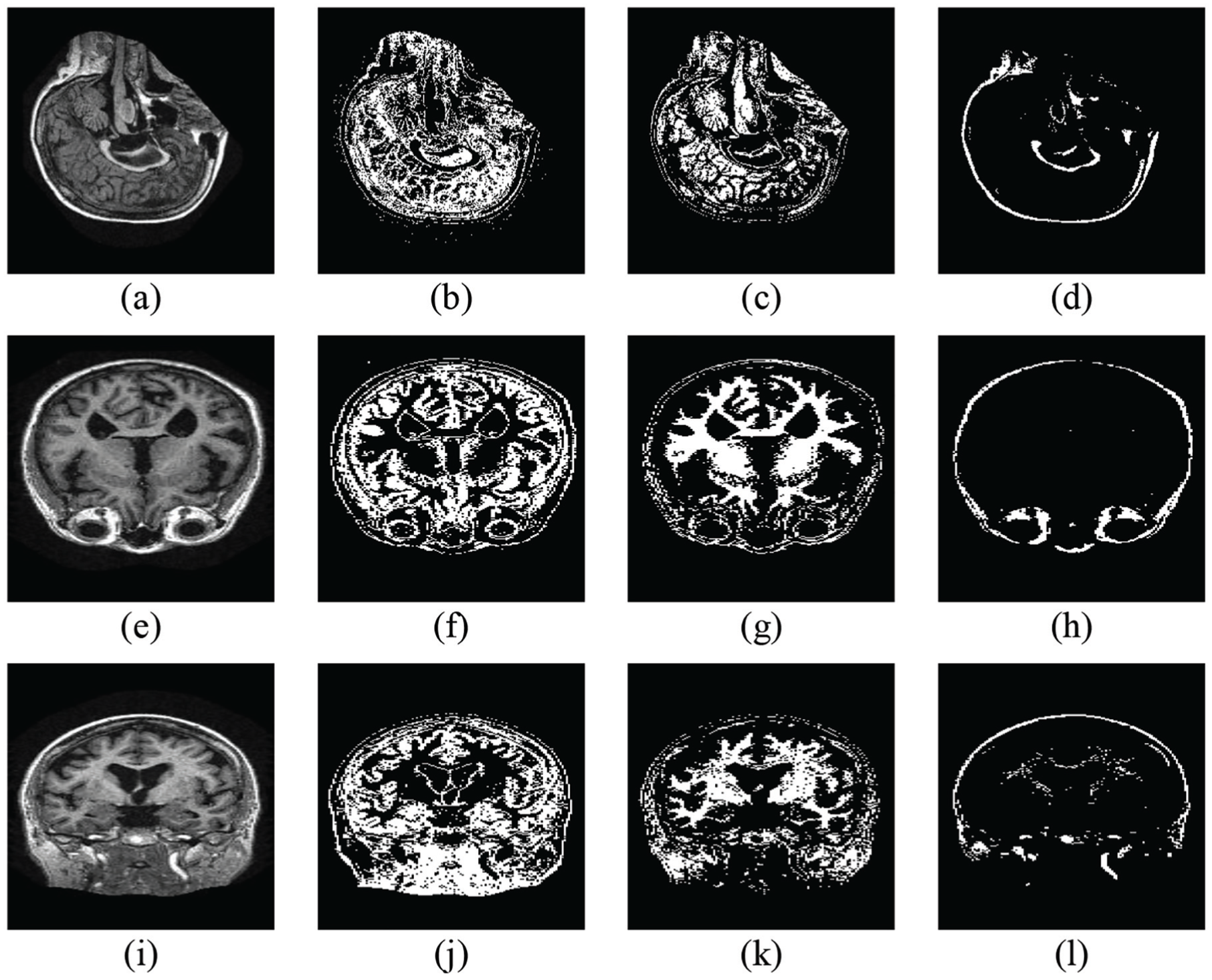
Image segmentation using multi-level thresholding: (a, e, i) the original images, (b, f, j) the GM, (c, g, k) the WM, and (d, h, l) the CSF segment.

An image-wise cumulative computational time graph shows the comparative analysis of our algorithm with the segmentation techniques of multi-level thresholding and K-means clustering in Figure 5.

Figure 5.

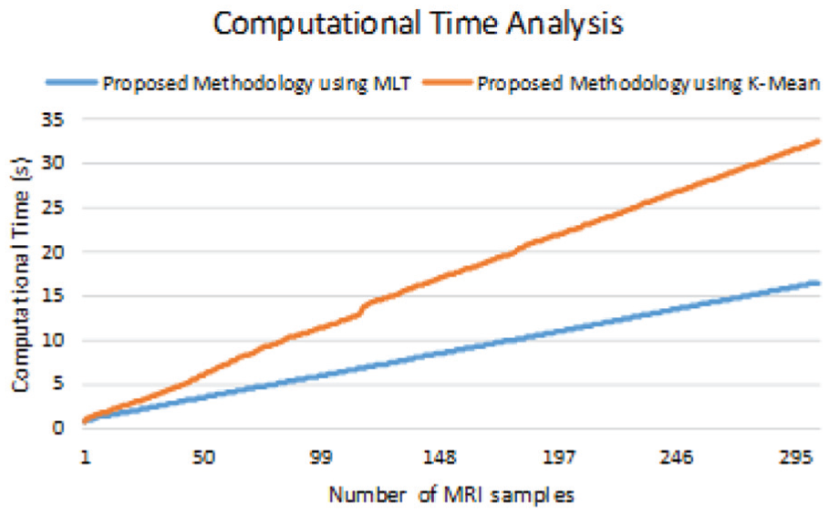
Comparative analysis of the proposed methodology using multi-level thresholding and K-means clustering.

Comparative analysis of other techniques

Binary and multi-class classifications of AD are of significant interest in the research community. Works have been done in the past few years in both binary and multi-class problems. A comparative analysis of the proposed method with the recent work done has been performed, as shown in Table 4.

Table 4.

Comparative analysis with binary classification techniques.

S. No.	Algorithm	Classifier	Accuracy (%)
1	The proposed algorithm	Random forest	99.2
2	MRI + clinical data	SVM	98.4
3	3D displacement field	SVM	93.05
4	GM volume reduction	SVM	83.17
5	GM volume reduction with feature ranking	SVM	92.48
6	Eigenshape descriptor–based model	KNN	93.37
7	Sparse regression model	N/A	71
8	Sulcal medial–based model	N/A	87.9
9	CHF-based feature model	N/A	62.07
10	CNN with auto-encoders	CNN	98.4

MRI: magnetic resonance imaging; 3D: three-dimensional; SVM: support vector machine; GM: gray matter; KNN: K-nearest neighbor; CHF: circular harmonic function; CNN: convolutional neural network. Bold values are the best results obtained in comparison to existing techniques.

S Wang et al. proposed a 3D displacement feature–based model which classified the test subjects by reducing the feature vector utilizing feature reduction algorithms. The images were classified with an overall accuracy of 93.05%. The method showed a high accuracy, which, however, left room for improvement. I Beheshti et al. proposed a method to detect AD based on the volume reduction of GM. Features were extracted from regions showing significant GM contraction and an overall accuracy of 84.17% was achieved. They followed a similar method reducing features based on feature ranking methodology resulting in a 92.48% accuracy. AK Ramaniharan et al. also proposed to detect Alzheimer’s based on the changing shape of the corpus callosum. The methodology showed promising results with an accuracy of 93.37%. These methodologies showed promising results; however, the significant change in the volume and shape can be detected through MRI scans only after the significant progression of the AD, due to which such methodologies are not practically feasible. A sparse regression model was also proposed showing an overall low accuracy of 71%.

M Plocharski and Østergaard proposed a sulcal medial surface–based feature model that was helpful in classifying the AD patients against the CN subjects. The model showed an overall accuracy of 87.9%. O Ben Ahmed et al. classified AD with an accuracy of 62.07%. The methodology utilized the harmonic functions as features. S Sarraf et al. proposed a convolutional network for a better classification accuracy reaching up to 98.4%. Tooba et al. utilized the MRI scans with clinical data and classified the textural features with an accuracy of 98.4%. In light of the given methods, a fully automated algorithm is proposed utilizing each view and segment of the human brain. A practically feasible algorithm was proposed dealing with the class imbalance problems in medical imaging. It resulted in an overall accuracy of 99.2% outperforming the rest of the techniques.

When it comes to multi-class classification, Alzheimer’s has not been detected and classified accurately. Accurate classification of different levels of dementia is of high significance predicting Alzheimer’s before progression into later stages. For that purpose, the literature showed a few implementations to achieve the accuracy as shown in Table 5. Tooba et al. performed a multi-class classification along with the binary one combining the textural features with the clinical data. The multi-class classification accuracy showed less promising results as compared to the binary one. An overall accuracy of 79.8% showed room for improvement. L Sørensen et al. used structural and morphological features like shape and thickness for multi-class classification and resulted in an accuracy of 62.7%. In contrast to the above algorithms, our proposed method showed equally good performance in multi-class Alzheimer’s classification. The technique utilized the 3D views combining the feature vector for accurate classification. Our algorithm outperformed the techniques to date with an accuracy of 99.025% under the naïve Bayesian classifier. Our proposed algorithm not only outperformed the existing ones in the literature in terms of accuracy but also processed the input MRI scan in an average time frame of 0.05 s. The low computational cost of our system ensures the feasibility of the smart CT scanners collecting MRI scans giving the classification results processed over the network. Our proposed algorithm utilized the IoT network architecture for the advanced methods to detect and classify MRI scans for the level of dementia in a patient dealing with the class imbalance problem.^36,37 The cross-domain research adds significance to our method by providing any efficient cloud-based diagnosis of Alzheimer’s.

Table 5.

Comparative analysis with multi-class classification techniques.

S. No.	Algorithm	Classifier	Accuracy (%)
1	The proposed algorithm	Multi-layer perceptron	99.025
2	MRI + clinical data	SVM	79.8
3	MRI + hybrid feature	LDA	62.7

MRI: magnetic resonance imaging; SVM: support vector machine; LDA: linear discriminant analysis.

Bold values are the best results obtained in comparison to existing techniques.

Conclusion

In this article, an IoMT-based decision system for AD was proposed. The system acquired the MRI scans of multiple patients over the network from smart CT scanners. The decision was made based on the proposed algorithm. For that purpose, a fully automated binary and multi-class Alzheimer’s classification model was proposed. The algorithm utilized the 3D views of the human brain MRI scan. It incorporated the GM, WM, and CSF segments collectively in the form of a super-feature vector over all three views. The algorithm also reduced the computational complexity by selecting the principal components for feature selection. The algorithm dealt with the class imbalance problem in medical imagery resulting in a promising accuracy of 99.2% in binary classification, while giving 99.025% in multi-class classification. The proposed methodology overcame the shortcomings and drawbacks in the reviewed literature. It also presented an IoMT-based approach to facilitate automated detection of Alzheimer’s in patients in remote locations. In future, we will be looking forward to utilizing standard state-of-the-art segmentation techniques like K-means. We will also be incorporating the clinical data with the MRI scans for high accuracy.

Footnotes

Handling Editor: Francesco Longo

Declaration of conflicting interests

The author(s) declared no potential conflicts of interest with respect to the research, authorship, and/or publication of this article.

Funding

The author(s) disclosed receipt of the following financial support for the research, authorship, and/or publication of this article: This study was supported by the MSIT (Ministry of Science, ICT), Korea, under the ITRC (Information Technology Research Center) support program (IITP-2019-2016-0-00312) supervised by the IITP (Institute for Information and Communications Technology Promotion).

ORCID iDs

Farhan Aadil

Ran Baik

References

Beheshti

Maikusa

Matsuda

et al . Histogram-based feature extraction from individual gray matter similarity-matrix for Alzheimer’s disease classification. J Alzheimer’s Dis 2017; 55(4): 1571–1582.

Beheshti

Demirel

Feature-ranking-based Alzheimer’s disease classification from structural MRI. Magn Reson Imaging 2016; 34(3): 252–263.

Belleville

Fouquet

Duchesne

et al . Detecting early preclinical Alzheimer’s disease via cognition, neuropsychiatry and neuroimaging: qualitative review and recommendations for testing. J Alzheimer’s Dis 2014; 42: S375–S382.

Wang

Zhang

Liu

et al . Detection of Alzheimer’s disease by three-dimensional displacement field estimation in structural magnetic resonance imaging. J Alzheimer’s Dis 2015; 50(1): 233–248.

Zhang

Wang

Phillips

et al . Detection of Alzheimer’s disease and mild cognitive impairment based on structural volumetric MR images using 3D-DWT and WTA-KSVM trained by PSOTVAC. Biomed Signal Process Control 2015; 21: 58–73.

Liu

Teverovskiy

Carmichael

et al . Discriminative MR image feature analysis for automatic schizophrenia and Alzheimer’s disease classification. In: Barillot

Haynor

Hellier

(eds) Medical image computing and computer-assisted intervention. London: Springer, 2004, pp.393–401.

Lao

Shen

Xue

et al . Morphological classification of brains via high-dimensional shape transformations and machine learning methods. Neuroimage 2004; 21(1): 46–57.

Stoeckel

Fung

. SVM feature selection for classification of SPECT images of Alzheimer’s disease using spatial information. In: Fifth IEEE international conference on data mining, Houston, TX, 27–30 November 2005, pp.410–417. New York: IEEE.

Klöppel

Stonnington

Chu

et al . Automatic classification of MR scans in Alzheimer’s disease. Brain 20083; 131: 681–689.

10.

Chincarini

Bosco

Calvini

et al . Local MRI analysis approach in the diagnosis of early and prodromal Alzheimer’s disease. Neuroimage 20112; 58: 469–480.

11.

Westman

Cavallin

Muehlboeck

et al . Sensitivity and specificity of medial temporal lobe visual ratings and multivariate regional MRI classification in Alzheimer’s disease. PLoS ONE 2011; 6(7): e22506.

12.

Ben Ahmed

Benois-Pineau

Ben Amar

et al . Classification of Alzheimer’s disease subjects from MRI using hippocampal visual features. J Multimedia Tools Appl 2014; 74: 1249–1266.

13.

Beheshti

Demirel

Matsuda

Classification of Alzheimer’s disease and prediction of mild cognitive impairment-to-Alzheimer’s conversion from structural magnetic resource imaging using feature ranking and a genetic algorithm. Comput Biol Med 2017; 83: 109–119.

14.

Beheshti

Demirel

Farokhian

et al . Structural MRI-based detection of Alzheimer’s disease using feature ranking and classification error. Comput Methods Programs Biomed 2016; 137: 177–193.

15.

Ramaniharan

Manoharan

Swaminathan

Laplace Beltrami Eigen value based classification of normal and Alzheimer MR images using parametric and non-parametric classifiers. Expert Syst Appl 2016; 59: 208–216.

16.

Guerrero

Wolz

Rao

et al . Manifold population modeling as a neuro-imaging biomarker: application to ADNI and ADNI-GO. Neuroimage 2014; 94: 275–286.

17.

Plocharski

Østergaard

LR.

Extraction of sulcal medial surface and classification of Alzheimer’s disease using sulcal features. Comput Methods Programs Biomed 2016; 133: 35–44.

18.

Ahmed

Mizotin

Benois-Pineau

et al . Alzheimer’s disease diagnosis on structural MR images using circular harmonic functions descriptors on hippocampus and posterior cingulate cortex. Comput Med Imaging Graph 2015; 44: 13–25.

19.

Sarraf

DeSouza

Anderson

et al . DeepAD: Alzheimer’s disease classification via deep convolutional neural networks using MRI and fMRI, 2016, https://www.biorxiv.org/content/10.1101/070441v4

20.

Sørensen

Igel

Pai

et al . Differential diagnosis of mild cognitive impairment and Alzheimer’s disease using structural MRI cortical thickness, hippocampal shape, hippocampal texture and volumetry. Neuroimage Clin 2017; 13: 470–482.

21.

Tooba

Anwar

Gul

et al . Multi-class Alzheimer’s disease classification using image and clinical features. Biomed Signal Process Control 2018; 43: 64–74.

22.

Battish

Analysis of pre-processing methods using MRI images. Analysis 2017; 5(2) [online].

23.

Kaur

Choudhary

Comparison of several contrast stretching techniques on acute leukemia images. Int J Eng Innov Technol 2012; 2(1): 332–335.

24.

Huang

Lin

WC.

Automatic multilevel thresholding based on two-stage Otsu’s method with cluster determination by valley estimation. Int J Innov Comput Inf Control 2011; 7(10): 5631–5644.

25.

Uma

JSS

. Human interaction pattern mining using enhanced artificial bee colony algorithm. Int J Innov Res Comput Commun Eng 2015; 3(10): 10131–10138.

26.

Mohanaiah

Sathyanarayana

Gurukumar

Image texture feature extraction using GLCM approach. Int J Sci Res Publ 2013; 3(5): 1–5.

27.

Karami

Prasad

Shehata

Image matching using SIFT, SURF, BRIEF and ORB: performance comparison for distorted images, 2016, https://arxiv.org/abs/1710.02726

28.

Dalal

Triggs

. Histograms of oriented gradients for human detection. In: 2005 IEEE computer society conference on computer vision and pattern recognition, San Diego, CA, 20–25 June 2005, pp.886–893. New York: IEEE.

29.

Kalsoom

Maqsood

Ghazanfar

et al . A dimensionality reduction-based efficient software fault prediction using Fisher linear discriminant analysis (FLDA). New York: Springer, 2018.

30.

Cohen

Zhou

et al . Feature selection using principal feature analysis. In: Proceedings of the 15th international conference on multimedia, Augsburg, 25–29 September 2007, pp.301–304. New York: ACM.

31.

Vijayarani

Muthulakshmi

Comparative analysis of Bayes and Lazy classification algorithms. Int J Adv Res Comput Commun Eng 2013; 2(8): 3118–3124.

32.

Vijendra

Vasudeva

Parashar

HJ.

Recognition of text image using multilayer perceptron, 2016, https://arxiv.org/abs/1612.00625

33.

Biau

Analysis of a random forests model. J Machine Learn 2010; 13: 1063–1095.

34.

Marcus

Wang

Parker

et al . Cross-sectional data across the adult lifespan. J Cog Neurosci 2007; 19(9): 1498–1507.

35.

Shin

Xiujuan

et al . Brain tissue segmentation using fast T1 mapping. In: Proceedings of the international society for magnetic resonance in medicine, Honolulu, HI, 18–24 April 2009. Wiley online library.

36.

Zhang

Y-D

Zhang

Phillips

et al . Synthetic minority oversampling technique and fractal dimension for identifying multiple sclerosis. Fractals 2017; 25: 1740010.

37.

Zhang

Y-D

Zhao

Sun

et al . Smart pathological brain detection by synthetic minority oversampling technique, extreme learning machine and Jaya algorithm. Multimedia Tools Appl 2017; 77: 22629–22648.

Internet of Medical Things–based decision system for automated classification of Alzheimer’s using three-dimensional views of magnetic resonance imaging scans

Abstract

Keywords

Introduction

Related work

Binary classification techniques

Multi-class classification techniques

The proposed methodology

Image preprocessing

Linear contrast stretching

Image segmentation

Feature extraction

Statistical features

Mean

Standard deviation

Kurtosis

Skewness

Geometric mean

IQR

Textural features

Gray-level co-occurrence matrix

Contrast

Correlation

Homogeneity

Entropy

Speeded-up robust features

Shape-based features—histogram of gradients

The class imbalance problem

SMOTE

Feature selection

PCA

Classification

BayesNet

Naïve Bayesian classifier

MLP

RF

Experimentation and results

Dataset

Accuracy assessment

Experimental setup

Results and discussion

Performance evaluation in terms of binary classification

Performance evaluation in terms of multi-class classification

Comparative analysis of our proposed system with the use of K-means clustering

Comparative analysis of other techniques

Conclusion

Footnotes

Declaration of conflicting interests

Funding

ORCID iDs

References