Dog recognition in public places based on convolutional neural network

Abstract

With the increase in the number of dogs in the city, the dogs can be seen everywhere in public places. At the same time, more and more stray dogs appear in public places where dogs are prohibited, which has a certain impact on the city environment and personal safety. In view of this, we propose a novel algorithm that combines dense–scale invariant feature transform and convolutional neural network to solve dog recognition problems in public places. First, the image is divided into several grids; then, the dense–scale invariant feature transform algorithm is used to split and combine the descriptors, and the channel information of the eight directions of the image is extracted as the input of the convolutional neural network; and finally, we design a convolutional neural network based on Adam optimization algorithm and cross-entropy to identify the dog species. The experimental results show that the algorithm can fully combine the advantages of dense–scale invariant feature transform and convolutional neural network to achieve dog recognition in public places, and the correct rate is 94.2%.

Introduction

With the improvement of people’s living standards, more and more people are starting to raise dogs. Residential areas and parks are a great place to take your dog. There is no need for the dog owner to worry about joggers, kids on bikes, and inattentive drivers. Like any recreational area, however, dogs are still at risk in public places. People and dogs get injured in dog parks throughout the United States. ¹ Unneutered male dogs and fearful dogs can be dangerous, because they might fight or bite as a fear reaction. Dog owners do not clean up after their dogs, which can cause the spread of disease. In 2018, a student from Xiangtan University was bitten by many stray dogs on campus. ² After the incident was published on the Internet, it caused a great public opinion storm. For this reason, the reputation of Xiangtan University also caused certain negative impacts. As we all know, researchers have more research on face recognition in public areas, but little attention has been paid to dog recognition in public places. Therefore, we propose a dog recognition algorithm that can help managers in public places. For residential areas, schools, parks, and other areas that prohibit dogs, the safety factor of these areas can be significantly improved.

Dog detection in public places falls within the scope of target detection. Compared to face detection, dog detection has greater inter-species differences and is more challenging in pattern recognition. Y Zhang et al. ³ proposed an algorithm for dog detection in an elevator. The algorithm was based on stacked autoencoder (SAE), combined with histogram of oriented gradient (HOG) to characterize the dog’s features. S Kumar and SK Singh ⁴ proposed a fusion-based pet identification method to identify dogs by biometrics. H Perez-Espinosa et al. ⁵ used dog-sounding to identify dog species through machine learning. AA Mohamed et al. ⁶ proposed a novel face recognition technique based on discrete wavelet transformed and local binary pattern (LBP) with adapted threshold to recognize avatar faces in different virtual worlds. They all achieved good results. However, they were not in the public field environment for dog species detection, which had certain limitations.

In particular environment of public places, we propose a public place dog recognition algorithm based on convolutional neural networks. First, the image is divided into several grids; then the dense–scale invariant feature transform (SIFT) algorithm is used to split and combine the descriptors, and the channel information of the eight directions of the image is extracted as the input of the convolutional neural network (CNN); and finally, we design a CNN based on Adam optimization algorithm and cross-entropy to identify the dog species. The algorithm has achieved good results in both time and space.

Dense-SIFT feature extraction

Feature extraction of images is one of the important steps in image classification. The quality of image feature extraction directly affects the performance of image classification. DG Lowe ⁷ proposed the image local feature extraction SIFT algorithm, which was widely used in image matching, object recognition, and other fields. After this, Lazebnik ⁸ proposed an improved SIFT feature extraction algorithm dense-SIFT. The method first used the pre-set grid size and sampling step size, then traversed the image from top to bottom and from left to right, and finally, extracted the SIFT features of each image block to form a feature descriptor. The motivation of the dense-SIFT feature extraction is that dense-SIFT can extract the features of the image in eight directions in advance, which helps to improve the performance of the CNN model. Therefore, we chose to use the dense-SIFT algorithm to process the image. The steps for dense-SIFT feature extraction are as follows:

• 1. Divide the image into several equal-sized grids.

We divide the original image (m pixels × m pixels) into regions of size x and remove the regions with less than x pixels, which gives $(m-x)/x\times (m-x)/x$ grid images of size x × x.

• 2. SIFT feature extraction for each divided grid image.

The feature descriptor is obtained by performing feature extraction on each small rectangular block after division by SIFT algorithm. SIFT operators are rich in information and unique. It has the characteristics of being constant when the image is rotated, the intensity of the light changes, and the scale of the image changes. Moreover, it has strong robustness when the angle of view of the image changes and the target is occluded. DG Lowe ⁹ pointed out that the area around the feature points is divided into 4 × 4 sub-areas, and the SIFT descriptor has the best performance. At this time, each sub-area serves as a key point, and each key point has eight directions, so each feature descriptor is a vector of 16 × 8 = 128 dimensions.

• 3. Split and combine the descriptors.

First, we describe the key points and extract the dimensional information in the same direction. Then, the descriptors are combined according to their original positional relationship to form a 4 × 4 dimensional intermediate information; finally, we combine the intermediate information into the same position of the rectangular block relative to the original image, and the description information of $4(m-x)/x\times 4(m-x)/x$ dimension can be obtained. The descriptor is split, as shown in Figure 1.

Figure 1.

The descriptor is split.

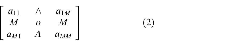
We extract the dimensional information of the 128-dimensional descriptors in the same direction and combine them according to their original positional relationships to form a 4 × 4 dimensional intermediate information. Its matrix representation (equation (1)) is as follows

$$\left[\begin{array}{cccc}{a}_{11}\hfill & a_{12}\hfill & a_{13}\hfill & a_{14}\hfill \\ \multicolumn{1}{c}{a_{21}}& a_{22}\hfill & a_{23}\hfill & a_{24}\hfill \\ \multicolumn{1}{c}{a_{31}}& a_{32}\hfill & a_{33}\hfill & a_{34}\hfill \\ \multicolumn{1}{c}{a_{41}}& a_{42}\hfill & a_{43}\hfill & a_{44}\hfill \end{array}\right]$$

(1)

After the descriptors are normalized, the value of each dimension is not greater than 1. Since the descriptor has direction information, no negative values will occur $(0\le a_{\mathrm{ij}}\le 1)$ . By performing the same splitting of $4(m-x)/x\times 4(m-x)/x$ descriptors, we can get $4(m-x)/x\times 4(m-x)/x$ 4 × 4 dimensional intermediate information. The 4 × 4 dimensional intermediate information of each small rectangular block is placed to the same position of the rectangular block relative to the original image. We can get a description of the $[4(m-x)/x]\times [4(m-x)/x]$ dimension. Its matrix representation (equation (2)) is as follows

$$\left[\begin{array}{ccc}\begin{array}{c}{a}_{11}\hfill \\ \multicolumn{1}{c}{M}\\ \multicolumn{1}{c}{a_{M1}}\end{array}\hfill & \begin{array}{c}\wedge \hfill \\ \multicolumn{1}{c}{o}\\ \multicolumn{1}{c}{\Lambda }\end{array}\hfill & \begin{array}{c}{a}_{1M}\hfill \\ \multicolumn{1}{c}{M}\\ \multicolumn{1}{c}{a_{\mathrm{MM}}}\end{array}\hfill \end{array}\right]$$

(2)

This is equivalent to the gray level information of a dimension image with resolution of $[4(m-x)/x]\times [4(m-x)/x]$ dimension, which can be used as input of CNN. If the feature maps in each direction are split and combined in the same way, then we can get the grayscale information of eight pictures. These eight grayscale images will be the input to the CNN. The algorithm flow is shown in Figure 2.

Figure 2.

Dense-SIFT feature extraction algorithm flow.

Construction of dog species recognition model based on CNN

CNNs are the most commonly used algorithms in image recognition, which have also achieved remarkable results in the fields of speech recognition, text analysis, and video processing. Mainstream CNN models such as LeNet, ¹⁰ VGGNet, ¹¹ and InceptionNet ¹² are mostly based on RGB three-channel image input. Few models use eight-channel pictures as CNN inputs. So, for the eight-channel image input, we have carefully designed a CNN model. The network structure is given in Figure 3.

Figure 3.

Convolutional neural network structure.

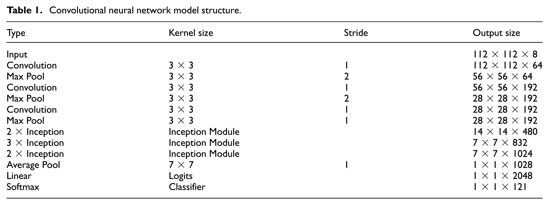
After the dense-SIFT algorithm extracts features, the image feature size is 112 × 112 × 8.

• The first layer: convolution layer; the size of the convolution kernel is 3 × 3; the convolution kernel has a step size of 1; the feature number is 64; the activation function is ReLU; and its output characteristic is 112 × 112 × 64.

• The second layer: Max Pool layer; the largest pooling layer; the size of kernel is 3 × 3; a step size of 2; feature output of 56 × 56 × 64; using batch normalization for the output. ¹³ Batch normalization was a technique for improving the performance and stability of artificial neural networks. It was a technique to provide any layer in a neural network with inputs that were zero mean/unit variance. It was used to normalize the input layer by adjusting and scaling the activations. For a layer with d-dimensional input x = (x(1),…, x(d)), we normalize each dimension

$${\hat{x}}^{(k)}=\frac{x^{(k)}-E[x^{(k)}]}{\sqrt{\mathrm{Var}[x^{(k)}]}}$$

(3)

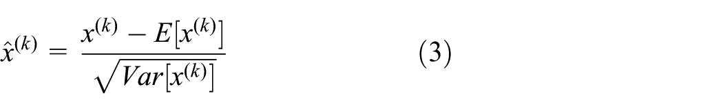
We introduce, for each activation $x^{(k)}$ , a pair of parameters ${\lambda }^{(k)}$ and ${\beta }^{(k)}$ , which scale and shift the normalized value

$$y^{(k)}={\lambda }^{(k)}{\hat{x}}^{(k)}+{\beta }^{(k)}$$

(4)

These parameters were learned along with the original model parameters and restored the representation power of the network.

• The third layer: convolution layer; the size of the convolution kernel is 3 × 3; the convolution kernel has a step size of 1; the feature number is 192; the activation function is ReLU; and its output characteristic is 56 × 56 × 192.

• The fourth layer: the largest pooling layer; the size of the core is 3 × 3; the step size is 2; the characteristic output is 28 × 28 × 192; using batch normalization for the output.

• The fifth layer: convolution layer; the size of the convolution kernel is 3 × 3; the step size of the convolution kernel is 1; the feature number is 192; the activation function is ReLU; and its output characteristic is 28 × 28 × 192.

• The sixth layer: Max Pool layer; the size of the core is 3 × 3; the step size is 1; the characteristic output is 28 × 28 × 192; using batch normalization for the output.

• The seventh layer: two Inception Module ¹² layers, using different scale convolution kernels to deal with features. The four results are connected and the total number of features obtained is 14 × 14 × 280.

The following levels are the same. Finally, through the average pooling layer, the linear layer, and the Softmax layer, we can get 121 categories. Detailed network model parameters are shown in Table 1.

Table 1.

Convolutional neural network model structure.

Type	Kernel size	Stride	Output size
Input			112 × 112 × 8
Convolution	3 × 3	1	112 × 112 × 64
Max Pool	3 × 3	2	56 × 56 × 64
Convolution	3 × 3	1	56 × 56 × 192
Max Pool	3 × 3	2	28 × 28 × 192
Convolution	3 × 3	1	28 × 28 × 192
Max Pool	3 × 3	1	28 × 28 × 192
2 × Inception	Inception Module		14 × 14 × 480
3 × Inception	Inception Module		7 × 7 × 832
2 × Inception	Inception Module		7 × 7 × 1024
Average Pool	7 × 7	1	1 × 1 × 1028
Linear	Logits		1 × 1 × 2048
Softmax	Classifier		1 × 1 × 121

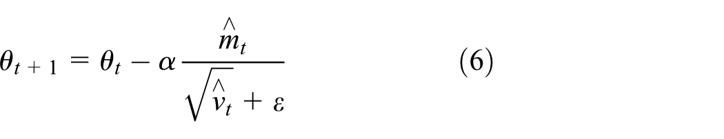
The Adam ¹⁴ optimization algorithm is an extension of the stochastic gradient descent algorithm, which uses the first-order moment estimation and the second-order moment estimation of the gradient to dynamically adjust the learning rate of each parameter. In the back propagation neural network (BPNN) process of Adam, after the offset correction, each iteration’s learning rate has a certain range, which makes the parameters relatively stable. So, we use the Adam optimization algorithm as the BPNN algorithm (equation (5))

$$\begin{array}{c}{m}_t={\beta }_1{m}_{t-1}+(1-{\beta }_1)g_t,v_t={\beta }_2{v}_{t-1}+(1-{\beta }_2)g_t^2\hfill \\ {\hat{m}}_t=\frac{m_t}{1-{\beta }_1^t},{\hat{v}}_t=\frac{v_t}{1-{\beta }_2^t}\hfill \end{array}$$

(5)

where $m_t$ and $v_t$ are the first-order matrix estimation and the second-order moment estimation for the shaving at time t, respectively; ${\hat{m}}_t$ and ${\hat{v}}_t$ are the deviation corrections for the $m_t$ and $v_t$ parameters, respectively; $\alpha$ is the learning rate of the model; ε is the smoothing term used to avoid the denominator being 0 and taking 1e−8. According to the recommendation of Kingma and Ba, ¹⁴ we set ${\beta }_1$ to 0.9; ${\beta }_2$ is set to 0.999; and the final formula ${\theta }_{t+1}$ is updated as follows

$${\theta }_{t+1}={\theta }_t-\alpha \frac{{m^{\wedge }}_t}{\sqrt{{v^{\wedge }}_t}+\epsilon }$$

(6)

The loss function is used to describe the accuracy of the model’s classification of the problem. The smaller the loss function, the smaller the deviation between the classification result of the model and the real data. We use cross-entropy as a loss function. Cross-entropy first appeared in information theory and is widely used in multi-classification problems, communication, error correction codes, and game theory. At the same time, in the loss function, the L2 regularization term is added to prevent over-fitting. The expression of the final loss function is as shown in equation (7), where ${\hat{y}}_i$ represents the predicted probability distribution, $y_i$ represents the true probability distribution, and $\lambda$ is the regular term coefficient

$$H(y)=-\sum _{i=1}^n{y}_i\log ({\hat{y}}_i)+\frac{\lambda }{2n}\sum _{j=1}^m||w_j|{|}^2$$

(7)

Experiment and analysis

Introduction to the experimental environment

The experimental environment and configuration are given in Table 2.

Table 2.

Experimental environment and configuration.

Environment	Configuration
OS	Ubuntu Server 14.04
Memory	16GB
CPU	Intel® Xeon® CPU E5-4603 v2
GPU	Matrox Electronic Systems Ltd
TensorFlow	1.3.0
CUDA	8.0
CUDANN	8.0.61

Experimental data

There are a lot of public data sets about dogs on the Internet, but the type, quantity, or size of these data sets is not in line with our expectations (lack of Chinese garden dogs). On the Internet, pictures of dogs in various categories are very rich. Therefore, we use Scrapy and Redis distributed crawler technology to crawl image data on the web and dry, crop, classify, and label the captured images. We have crawled the image data of 121 categories of dogs (see Appendix 1 for specific categories), 500 pictures per type, and the image size is 560 × 560. The images are shown in Figure 4.

Figure 4.

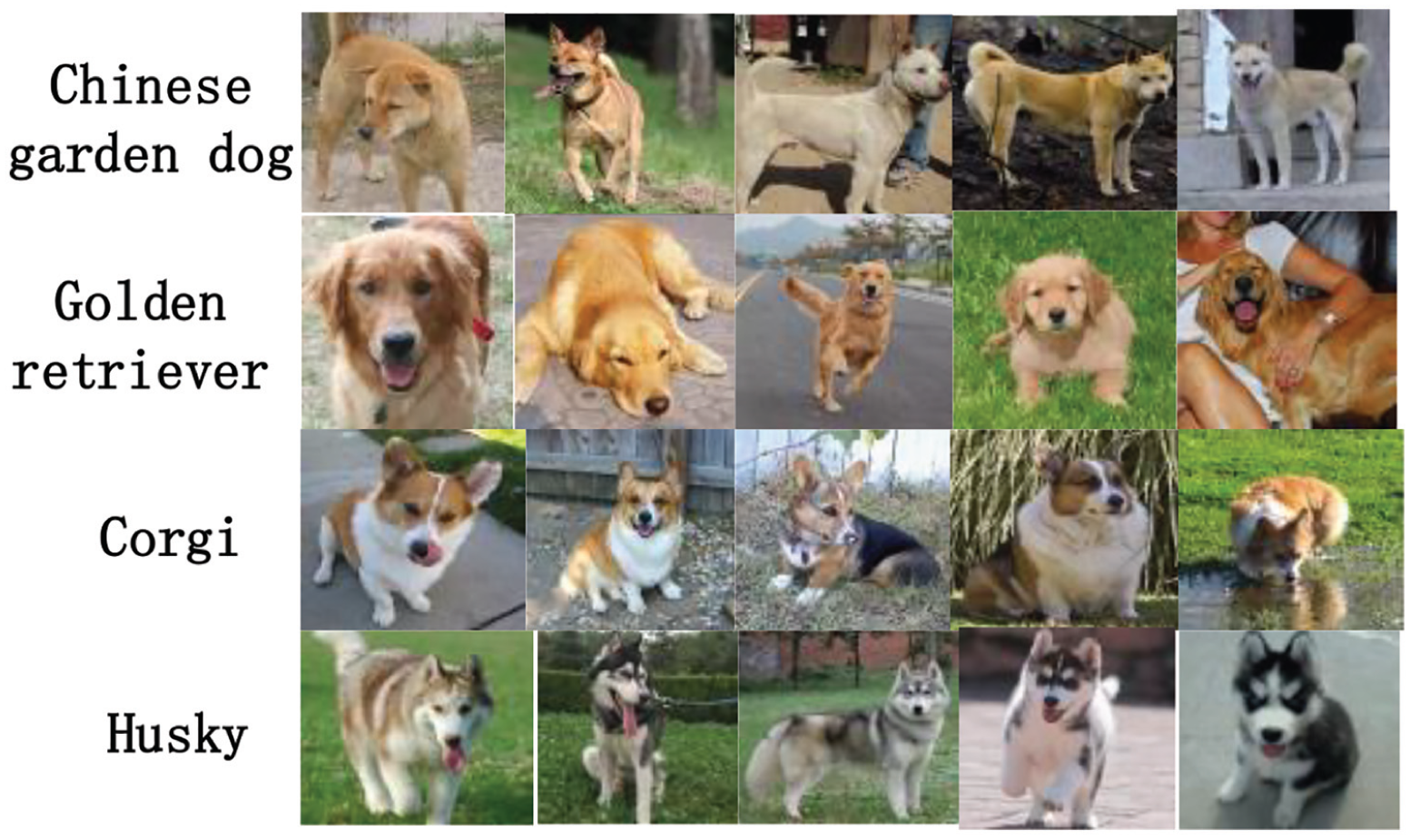
Part of the data set.

Experimental recognition results and analysis

The image is extracted and the features are split and combined. We set the step size of the image to 20 pixels, so a picture with a resolution of 560 × 560 will be divided into 28 × 28 small pictures with a size of 20 × 20. Using the dense-SIFT algorithm, 28 × 28 descriptors of 4 × 4 × 8 dimensional information can be obtained. For all descriptors, according to the split combination method in section “Dense-SIFT feature extraction,” we can get eight channels of grayscale images with an image resolution of (28 × 4) × (28 × 4) = 112 × 112. In the training process, 80% of the data are used as a training sample, 10% of the data are used as a test sample, and 10% of the data are used as a verification sample. We use 1e–4 learning rate training; the accuracy and loss function of the test sample are shown in Figure 5.

Figure 5.

Accuracy (left) and loss function (right) of the test set.

It can be seen from Figure 5 that the accuracy rate is basically rising during the whole training process. After 1000 iterations, the accuracy and loss functions gradually increase steadily, and the recognition rate is about 90%. The speed of convergence is mainly due to the Adam optimization algorithm, and then, after 2000 iterations, the final accuracy rate is 94.2%. The accuracy and loss function values of the validation set are shown in Figure 6.

Figure 6.

Accuracy (left) and loss function (right) of the validation set.

We can see that when the model is iterated to 3000 times, the accuracy of the verification set reaches the highest and the value of the loss function reaches the lowest. When the training accuracy continues to decrease, an over-fitting occurs. So, our model iterates 3000 times under the learning rate of 1e–4.

The experimental results were compared with models such as support vector machine (SVM), InceptionNet V3, VGGNet, and BPNN (three layers). The results are shown in Table 3.

Table 3.

Comparison of experimental results.

Method	Recognition time (s)	Recognition rate (%)
Ours	0.432	94.2
InceptionNet V3	0.663	85.7
VGGNet	0.871	83.4
SVM	0.470	80.8
BPNN (three layers)	0.028	70.6

SVM: support vector machine; BPNN: back propagation neural network.

In terms of recognition rate, the proposed method can achieve a correct recognition rate of 94.2%, benefiting from the feature extraction of dense-SIFT. Through the dense-SIFT algorithm, the picture of the eight directions of the picture is extracted, and the feature preprocessing is performed before inputting the neural network. In terms of recognition speed, the algorithm proposed in this article is better than InceptionNet V3 and VGGNet networks in time. The main reason is that the network model proposed by the text is less than InceptionNet V3 and VGGNet at the network level, so it also has certain advantages in recognition time.

Relationship between learning rate and recognition rate

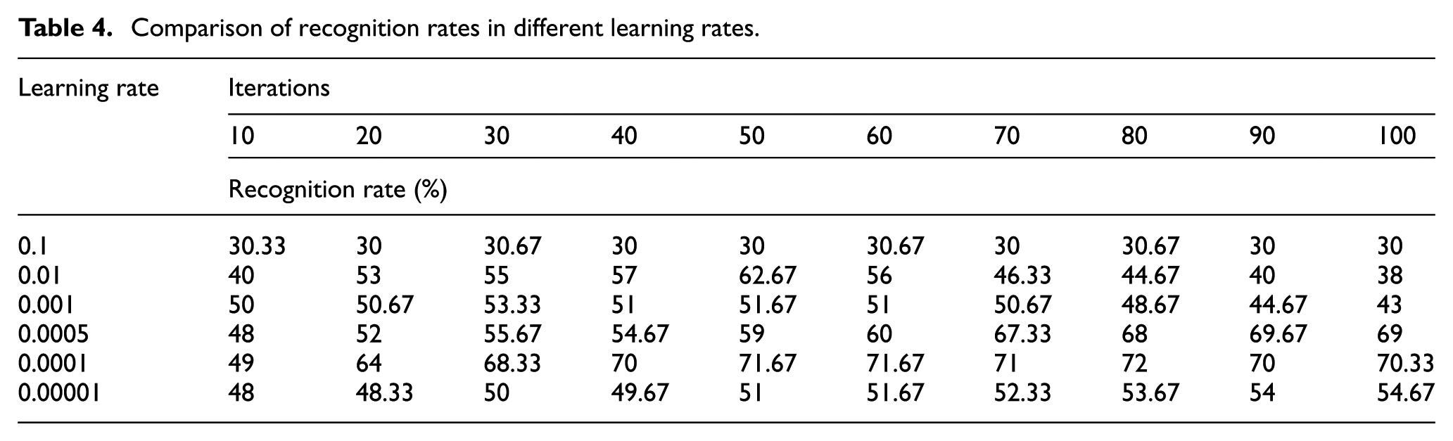
When the learning rate is set to 0.1, 0.01, 0.001, 0.0005, 0.0001, and 0.00001, the experimental results of the recognition rate are shown in Figure 7.

Figure 7.

Relationship between learning rate and recognition rate.

It can be seen from Table 4 that when the learning rate is 0.1, the recognition rate does not change substantially, which indicates that the feature cannot be effectively extracted at this time. When the learning rate is 0.01, the recognition rate is gradually increased before 50 iterations, but the recognition rate shows a downward trend after 50 iterations, indicating that over-fitting occurs after 50 iterations. When the learning rate is 0.001, the recognition rate can only reach 51%. When the learning rate is 0.00001, although the recognition rate does not appear over-fitting, it only reaches 54.67%. When the learning rate is 0.0001 and 0.0005, the recognition rate can be gradually increased and finally increased to about 70%, and there is no downward trend. This shows that both learning rates enable the network to perform effective feature extraction and learning without over-fitting. When the learning rate is 0.0001, the recognition rate is 70% only after 40 iterations. The learning rate is 0.0005, and the recognition rate is close to 70% when iteration is nearly 100 times. This shows that the network structure performance is better when the learning rate is 0.0001, so we choose the learning rate of 0.0001.

Table 4.

Comparison of recognition rates in different learning rates.

Learning rate	Iterations
	10	20	30	40	50	60	70	80	90	100
	Recognition rate (%)
0.1	30.33	30	30.67	30	30	30.67	30	30.67	30	30
0.01	40	53	55	57	62.67	56	46.33	44.67	40	38
0.001	50	50.67	53.33	51	51.67	51	50.67	48.67	44.67	43
0.0005	48	52	55.67	54.67	59	60	67.33	68	69.67	69
0.0001	49	64	68.33	70	71.67	71.67	71	72	70	70.33
0.00001	48	48.33	50	49.67	51	51.67	52.33	53.67	54	54.67

Summary and outlook

We studied the recognition of dogs in public places, designed a CNN model, and extracted the channel information of the eight directions of the image as the input of the CNN through the dense-SIFT extraction algorithm. We have achieved good results in accuracy and recognition time. The next work will continue to study in-depth from the following three aspects: (1) to improve the recognition speed and generalization ability of the feature model; (2) to detect the number and location of dogs; and (3) to test in bad weather.