Sage Journals: Discover world-class research

Abstract

Alzheimer’s is the main reason which leads to memory loss of a human being. The living style of an affected person also varies. This variation in the lifestyle creates difficulties for a person to spend a normal life. The detection of Alzheimer’s disease in the initial stage accurately has a great significance in the early treatment of the disease. Therefore, it is considered as a challenging task. An efficient method is proposed to detect the Alzheimer’s disease in the early stage using magnetic resonance imaging. k-Means clustering is used to develop the proposed method for efficient segmentation of the white matter, cerebrospinal fluid, and grey matter. The amalgam feature vectors are formed using the grey-level co-occurrence matrix and speeded-up robust features based on textural feature extraction. Statistical and histogram of gradients is used from shape-based features. Fisher linear discriminant analysis is used for dimensionality reduction and the resampling method is used to handle the class imbalance problem. The algorithm is evaluated using the three classifiers k-nearest neighbour, support vector machine and random forest. The dataset of OASIS is used to assess the outcomes. The proposed approach achieved the optimum accuracy of 92.7%.

Keywords

Alzheimer’s detection class imbalance learning histogram of gradients Fisher linear discriminant analysis

Introduction

Alzheimer’s disease (AD) is a problem in which a normal person loses the ability to do daily routine tasks. This occurs due to the disorder of the neurological brain. Afterward, it damages the brain cells.^1,2 The proportion of population affected by this disease is increasing day by day and, according to researchers, it will reach about 16 million in the coming years.³ As the proper reason and cause of this disease are not identified, distinguished treatment methods cannot be found and research is still in progress.^4,5 Nevertheless, the detection of AD in its initial stage is considered fruitful for the patient as early diagnosis leads to early treatment. Alongside the growing age, the functional abilities of the patient will be restored for a longer period. The detection of AD is a challenging task in which neuroimaging data help to accurately sense the disease in its early stage. Mild cognitive impairment (MCI) is the terminology used to define the early stage of AD. It means that AD is developing or that an attack is about to occur. MCI has a 10% conversion rate to AD.⁶

Magnetic resonance imaging (MRI) is used to obtain the accurate image of the body with high approachability, good contrast, and high resolution.^1,2 The region of interest (ROI) and volume of interest (VOI) are used for the classification and extraction of features. These factors are used for the measurement of the hippocampus, the medial temporal lobe, and grey matter (GM) voxels in the segmented images.^3,7–9 The detection of MCI is considered as the challenging task nowadays. There are so many factors which are used to find AD. Some of them are clinical dementia rate (CDR), mini-mental state examination (MMSE), complete patient history and neurobiological exams. The resting-state functional magnetic resonance imaging (rs-fMRI) and structural MRI are used to study the brain condition such as hippocampus, ventricle enlargement in the brain and cerebral cortex shrinks because of AD. These factors affect the brains for planning, thinking, memory and so on. The stage of the disease is proportional to the change of the brain areas. The changes in the brain parts such as the cerebral cortex and hippocampus are easily detectable using MRI.¹⁰ Nowadays, a lot of research is in progress on this disease and better results are being obtained.¹¹ It still requires vast knowledge to find AD by observing the MRI. For that, the other factors as mentioned earlier also should be kept in mind to detect AD. There are multiple stages of AD and to develop an efficient technique for multiclass classification remains an open research question.^5,12–14 Apart from the MRI scans, electroencephalogram (EEG) tests are also performed to diagnose the neurological condition of the patient. Works have been done by some researchers;^15–20 however, it is also challenged with the spatial resolution, that is, it is a challenging task to determine the depth of the incoming brain signals.

In this article, we propose a texture-based classification method for Alzheimer’s detection from the MR images. The idea is to segment out different sections of MR images based on intensity. An improved k-means clustering technique is used to separate out the white matter (WM), GM and cerebrospinal fluid (CSF). A hybrid feature vector is extracted from each segment separately and combined to form a single vector. The feature vector consists of textural, statistical and shape-based features. The textural features are grey-level co-occurrence matrix (GLCM) and speeded-up robust features (SURF), while shape-based features consist of histogram of gradients (HoG).

A Fisher linear discriminant analysis (FLDA)–based dimensionality reduction technique is used to select the discriminative features. As the number of instances for each stage of Alzheimer’s is not comparable, it also faces the class imbalance problem and resampling with a substitute is used to handle this problem. We have used the OASIS dataset to evaluate the performance of the proposed method. The results show the superiority of the proposed method. This work proposes the following key points:

A hybrid feature vector based on textural, statistical and shape-based features;

The use of an improved k-means algorithm to segment out the WM, GM and CSF;

The FLDA-based dimensionality reduction technique to select discriminative features for Alzheimer’s detection.

The remainder of this article is organized as follows: section ‘Related work’ presents the related work, section ‘The proposed methodology’ explains the methodology and section ‘Experimentation and results’ presents the results followed by a conclusion and future work.

Related work

Beheshti et al.⁸ proposed a method where images were segmented into GM, WM and CSF in the first step among the five. In the second step, GM segmented ROIs to generate similarity matrices. In the third step, statistical features were obtained. Statistical features and clinical data have been merged in the last two steps. Functional activities questionnaire and support vector machine (SVM) classifier were used for the classification of data in the AD versus normal group. S Wang et al.³ utilized three-dimensional (3D) field estimation–based method to classify the AD and normal patients. The classification was done by an SVM classifier and an accuracy of 93.05% was obtained. The VOIs were segmented by Beheshti et al.²¹ from the parts that have a noteworthy GM volume reduction. From these voxel values, a feature vector was extracted and the ranking was done using the genetic algorithm and t-test scores. This was done so that an optimal subset of features could be selected. SVM with a 10-fold cross-validation was utilized for performing classification. The accuracies of 84.17% and 70.38% were obtained for Alzheimer’s versus normal and mild versus normal, respectively.

In Beheshti et al.,⁵ voxel-based morphometry (VBM) was used to determine the GM volume in AD patients and healthy controls. Portions with significant and enormous GM atrophy changes were picked and selected as VOIs. As raw features, voxel values from these portions were selected. Later, these values were evaluated using seven feature ranking techniques. SVM was used as a classification technique and achieved 92.48% accuracy. AK Ramaniharan et al.¹⁰ proposed an algorithm to use a Laplace eigenvalue shape descriptor for the sake of classification of AD. In order to select the most significant features, information gain ranking was used and these were classified using k-nearest neighbour (KNN) and SVM. The KNN classifier yielded the accuracy of 93.37%. Quantifying variations in the microstructure of the corpus callosum is not an easy task and hence it makes this technique not so useful in practice.

R Guerrero et al.²² proposed a structure that shows inter-subject variability for feature extraction from low-dimensional sub-spaces. To create manifold space, data-driven ROIs were used and, to learn these regions, a sparse regression with the MMSE score was used. For variable selection, sampling bias was reduced with the resampling scheme with sparse regression. A classification accuracy of up to 71% was attained. A sulcal medical surface for the AD and cognitively normal classification was put forward by M Plocharski and LR Østergaard¹² and a classification accuracy of up to 87.9% was obtained. Certain other measurements like cortical thickness, hippocampus texture and shape were merged by L Sørensen et al.⁴ to form a biomarker which used information from the MRI data. For the aforementioned technique, linear discriminant analysis (LDA) was trained for Alzheimer’s Disease Neuroimaging Initiative (ADNI). According to the results, combinational MRI biomarkers achieve a 62.7% multiclass classification accuracy. S Sarraf et al.²³ proposed a method, in which local features were obtained by circular harmonic features from the hippocampus and posterior cingulate cortex. The accuracy of 62.07% was achieved for AD versus MCI.

In S Sarraf et al.,²³ a deep learning algorithm was proposed for Alzheimer’s detection. A combination of convolution neural networks with auto-encoders was used for binary classification of Alzheimer’s. A classification accuracy of 98.4% was achieved and another multiclass classification was not included. For the extraction of discriminative features, a convolution neural network was used to classify the AD and normal subjects.²⁴ Deep learning–based methods show great results in big data analysis, but collecting relevant information from huge and unstructured data needs a great deal of training, whereas selecting optimal hyperparameters and suitable architecture is not an easy task.²³

Another challenging task is the binary classification of AD and MCI. Also, multiclass classification including AD, normal and MCI is a difficult task. Most of the techniques mentioned in the literature emphasize the features directly extracted from the brain images. In this research, clinical information was utilized with features extracted as both whole and segmented brain images. This showed betterment in the performance of binary and multiclass classification.

Improvement of performance in both binary and multiclass classification is the aim in the development of automated detection systems. Some recent advancements in Ding et al.^25–27 show the improved methods that can be utilized among the classification stages resulting in the development of computationally intelligent systems.

The proposed methodology

The proposed technique (presented in Figure 1) is a multistep algorithm that takes simple MRI scan images as input and classifies them as having Alzheimer’s or not. The multiple steps of our proposed algorithm are explained in the sections below.

Figure 1.

The proposed methodology for multiclass Alzheimer’s classification.

Image preprocessing

MRI scans are taken using a large magnet and radio waves to have a look at the inner organs of a human being. Medical specialists utilize MRI technology for the diagnosis of the internal condition of the organs. MRI is proven to be very useful for the examination of the brain and spinal cord. During the formation of an MRI scan, it may get affected as it is susceptible to the environment. Images may get degraded due to luminance non-linearity or suffer from poor contrast due to the optical devices. To obtain better results, images are preprocessed using the image enhancement methods. For this purpose, the intensity of the image is adjusted and enhanced. Dynamic ranges can be adjusted by different methods among which contrast stretching is an efficient mode.

Contrast stretching

Contrast stretching also known as normalization is an image enhancement technique that works by attempting to improve an image by stretching its range of intensities.²⁸ The range of intensities is stretched to the new limit making full use of the new possible values. In contrast to histogram stretching, it works by linearly mapping the input values to the output ones. Contrast stretching uses the possible values of the range and maps the old ones onto them expanding the range due to which small contours and details are highlighted. Any information that has not been highlighted in the input imagery may get enhanced during the process. Stepwise contrast stretching is performed as follows:

The new range of values (lower limit and upper limit) are determined as a and b, respectively, to which the image’s intensities will be expanded. For an 8-bit image, the range is usually from 0 to 255.

Histogram of the original image is calculated and its lower and higher limits c and d are determined.

Since it is a point operation, for each pixel value r the output value s is mapped as

s = (r - c) (\frac{b - a}{d - c}) + a

(1)

During the image formation of MRI scans due to an inadequate amount of light and improper light adjustment, images do get a poor contrast, due to which the histogram of the whole image is having a non-uniform distribution. Contrast stretching stretches the intensity distribution and enhances the obscured information in the darker region required in the later stages.

Here r is the input pixel value, a and b are the lowest and highest possible intensity levels to be represented in the 8-bit image, respectively, and c and d are the actual lowest and highest intensity levels in the input image, respectively.

Image segmentation

Image segmentation is the division of an image into multiple non-overlapping regions based on the intensity variations and contours. MRI scans capture the internal structure and components of the human brain. GM, WM and CSF are the components representing the compartmental model of the human brain. MRI scans capture these compartmental models in a single image. However, they vary in their representative intensities. This variation in their intensities makes them easy to be segmented into each of the model components. To segment the individual components, the k-means clustering technique is used grouping the pixels with similar intensity levels. The k-means clustering technique is discussed in the section below.

k-Means segmentation

k-Means clustering is an unsupervised learning algorithm used to group data points with similarities among them. This results in the formation of clusters of data points sharing similar attributes. When it comes to images, the data points are the pixels with intensity levels as their attribute. Each data point is represented by their feature vector; however, in this case, a single grey-scale value is used. The algorithm forms a group of pixels based on the distance between them. The distance is not based on their graphical separation but their tonal separation. The k-means algorithm takes the image as an input along with the number of clusters to be formed represented by k. Different methods are used to find the optimal value of k for better segmentation; however, it can also be determined by the visual interpretation of data.²⁹ Segmenting out the components of the compartmental model of the brain the value of k can easily be determined as the number of those components, that is, three. Once the input parameters are calculated and passed, the iterative algorithm of k-means is initiated. The steps performed over the iterative procedure are discussed below.

Centroid initialization is a key step towards achieving good segmentation results. It is the selection of data points as the initial cluster heads or centroids around which the rest of the data points will gather. The location of the centroids is of high significance and is usually required to be placed far apart from one another. The k-means algorithm utilizes the cluster centroid initialization through a random process. In our proposed system, k-means clustering using centroid selection through a heuristic function has been used. It is observed that the centroids initialized through the heuristic function show an improvement in performance and efficiency. The heuristic function used for centroid initialization is given as

μ_{i} = i * \frac{m}{k + 1}

(2)

where m is the maximum intensity value, k is the number of clusters and i iterates from 1 to k. The preprocessed images with contrast stretched to the maximum limits of an 8-bit image make the value of m 255. A data point, in this case a pixel, is assigned to a cluster based on the distance between the pixel and the k cluster centroids. Pixel is assigned to the cluster whose distance comes out to be the minimum, as a result of which similar intensities are grouped together into a single cluster resulting in forming a single segment. The distance between the pixel and its k-centroids is given as

C_{i} = arg min x_{i} - μ_{j}

(3)

where $C_{i}$ is the cluster label for the pixel i based on the minimum distance between the pixel $x_{i}$ and the centroids, $μ_{j}$ . Once the labels are assigned to each pixel of the image, new centroids are found for the next iteration. These centroids are not found randomly or through some heuristic function but as a mean of the pixels with label i. The mean values found in this result will be used as the new centroids in the next step. The centroids are recalculated and updated as

μ_{i} = \frac{\sum_{i = 1}^{m} l {C_{i} = j} x_{i}}{\sum_{i = 1}^{m} l {C_{i} = j}}

(4)

where i iterates over the number of pixels and j iterates over the number of clusters k. The iterative algorithm comes to an end when the variation in the centroid values stops. During the iterative procedure, the centroids are recalculated moving to their final position. Once the values of centroids come out to be the same as the previous one, clustering comes to an end.

Feature extraction

Feature extraction is one the most important steps in the multistep classification system. The accuracy of the system is based on how many relevant and characteristic features are used.^28–30 Our proposed methodology utilizes the compartmental components of the brain, that is, GM, WM and CSF for the detection of AD. Thus, each component undergoes feature extraction separately. To distinguish between the images of patients with different levels of Alzheimer’s along with the healthy subject characteristics, a feature vector is required. For this purpose, different feature extraction techniques are used. To incorporate features from different domains, feature extraction techniques under such domains are considered. Statistical, textural and shape-based features are extracted from the input segmented images of GM, WM and CSF.

Statistical features

They include features based on the image histogram. An image histogram is a graphical representation of the distribution of intensity levels along with their frequency. It gives the occurrence of each pixel value in the image and an overview of the number of intensity levels in that image. Segmented regions of GM, WM and CSF are characterized by their distinctive intensity levels, thus each having a unique histogram. The histogram of the segments is plotted, and the first-order statistical information is extracted. Features such as mean, standard deviation, kurtosis, and skewness. Each of the features is represented in Table 1. Here hist(i) is the histogram calculated for the pixel i and N is the total number of pixels.

Table 1.

Description of statistical features.

Serial No.	Feature	Description	Formula
1	Mean	Average value of the image	$μ = \sum_{i = 1}^{N} i . hist (i) / N$
2	Standard deviation	Amount of spread of intensity levels	$σ = \sqrt{(1 / N) \sum_{i = 1}^{N} {(i . hist (i) - μ)}^{2}}$
3	Kurtosis	Measurement of tailedness of data	$K = ((\sum_{i = 1}^{N} (i . hist (i) - μ)^{4}) / N) / σ^{4}$
5	Skewness	Symmetry of the histogram	$Sk = ((\sum_{i = 1}^{N} (i . hist (i) - μ)^{3}) / N) / σ^{3}$

Textural features

The texture is a key feature formed by the spatial arrangement of pixel values. It represents the relationship between the pixel values over a certain region. Each segment in the MRI scan has its distinctive intensity levels forming a distinctive relationship with the neighbouring pixels. Such a relationship is exploited in textural feature extraction techniques such as GLCM and SURF. Each of the technique is elaborated below.

A co-occurrence matrix over an image is the matrix representing the distributions of intensity levels in the image at a given location.⁹ It represents the spatial and angular relationship between the pixels over a specified region of the image. GLCM is the co-occurrence matrix that represents how often a pixel with a grey level with value i occurred horizontally, vertically or diagonally in the image with pixel with intensity j. The matrix is of size N × N where N is the number of intensity levels from 0 to N – 1. Considering an element of GLCM, P(i,j) contains the frequency with which pixels with values i and j have occurred together horizontally, vertically or diagonally in an image. The co-occurrence of the pixels is calculated over the entire image populating the co-occurrence matrix. The steps to calculate the GLCM are given as follows:

Initialize each position of the GLCM of size N × N with 0;

For the location of GLCM as (i,j), calculate the number of occurrences P(i,j) of pixels i and j together in the respective directions;

Repeat the above step for each location of GLCM.

Once the GLCM is formed different features are calculated. Those features are briefly discussed below.

Contrast is defined as the variation in different areas specified within GLCM. Mathematically, it is represented as

Contrast = \sum_{x, y} {| x - y |}^{2} \log P_{r, θ} (x, y)

(5)

where $P_{r, θ}$ is the co-occurrence matrix and (x,y) represents the transition of intensity levels from x to y.

Correlation is a measure of the cumulative probability of a pair of values occurring in the GLCM. Mathematically, it is given as

Correlation = \sum_{x, y} \frac{(x - μ_{1}) (y - μ_{2}) P_{r, θ} (x, y)}{σ_{1} σ_{2}}

(6)

where $μ_{1}$ and $μ_{2}$ are the means of two correlated images with standard deviations $σ_{1}$ and $σ_{2}$ , respectively.

Homogeneity is the quantified measurement of closeness between the GLCM elements and their diagonals. Mathematically, it is specified as

Homeogeneity = \sum_{x, y} \frac{P_{r, θ} (x, y)}{1 + {| x - y |}^{2}}

(7)

Entropy is the reciprocal measurement of the elements in the order in an image. The higher the entropy, the less the image is uniform. Mathematically it is given as

Entropy = - \sum_{x, y} P_{r, θ} (x, y) \log P_{r, θ} (x, y)

(8)

SURF is a textural feature extraction technique that works by applying Gaussian filtering over the image in a squared window manner.³⁰ The method detects the points of interest using the blob detector over the Hessian matrix. The filtering over the relatively small windows results in an efficient and robust filtering of the image than the normal filtering of the image. Once the points of interests are calculated, wavelet responses around the neighbourhood of those points are performed to obtain the feature descriptors of the image. SURF over the segmented MRI scans is performed providing multiple feature descriptors. Among the feature descriptors, the strongest ones are selected. Local features are then extracted around those points.

Shape-based features

Reduction of GM and variation in the shape of internal components of the brain are the key discriminative facts that can be used to detect Alzheimer’s in the test patients. The shape of the brain and its components are represented by the edges formed around the component giving the shape of it. Similarly, the ridges and folds of the brain are also extracted using the edges that form the distinctive shape. For that reason, the shape-based feature extraction technique is used to identify the shape descriptors.

Edges and contours in an image are formed by the variation in the intensity levels of an image. Such edges from around the shape of the image play the role of the shape descriptors.⁷ HoG is the distribution of the variation in the intensity levels within an image. It records the frequency distribution of grey-level variation in each direction with an offset of 45 degrees. The distribution is utilized to interpret the shapes formed by the variations in the intensity levels. HoG is a local feature extraction technique used to perform the operation over the window of size 8 × 8. The window is then slid over the entire image.

The individual features extracted over the segmented images from the original MRI are combined to form a single hybrid feature vector incorporating all the statistical, textural and morphological information required to accurately classify the levels of Alzheimer’s from the MRI scans of the test subjects. The hybrid feature vector not only combined the individual features together but also added the size of the individual features in it. Such a large feature space seems to have redundant features with no contribution to the distinctive property of the vector altogether. Also, it seemed to be inadequate for the classification algorithm in the latter step. To address the posed computational complexity due to a high-dimensional feature vector, the feature selection technique is utilized.

The class imbalance problem

It is a condition where the data samples from the classes are not uniformly distributed in terms of their number. Once the features are extracted and are fed into the classification stage, the data samples are normalized for appropriate classification results. Samples belonging to the minority class offer the least contribution in the calculation of the overall accuracy of a system. The system will still show high accuracy even though all the samples are misclassified due to its low weight in the result. This leads to ambiguous and faulty decisions by the detection systems. To address this problem, various techniques have been utilized. The techniques can be applied to the data perspective or algorithm perspective. Concerning the functionality of the algorithm, some techniques are applied with the data perspective. Resampling is proposed in our system.³¹

This method is based on the boot-strapping approach used to produce the data artificially instead of proper measurement. Several samples are obtained with and without the use of the replacement methods. It produces the class which is equally likely and solves the misbalancing problem. Similarly, in our case, the samples belong to different classes and are unequal. Therefore, this method produces oversampling for the class with a smaller number of samples, that is, minority class. Due to this, classifier bias is minimized by generating the equal ratio for all the existing classes. This helps solve the class imbalance problem in our proposed algorithm.

Feature selection

It is the process to find the features which are different from the others. Our main motive is to collect the different features from the image to obtain better results. The features are passed through the classifiers of machine learning. To achieve performance enhancement, we have used the dimensionality reduction method to reduce the number of features. This technique reduces the feature vector and selects the features which are distinctive than the others. FLDA is used for that purpose in which class labels are used to differentiate the different features.³² FLDA selects the subset of features that contribute to maximizing the intra-class variance leading to promising classification results, thus making FLDA the suitable feature selection technique reducing the high dimensionality of the input data.

Classification

Once the features are extracted, combined, reduced and normalized to overcome the class imbalance problem, the feature vector is then fed into the classification algorithms to detect and classify the level of Alzheimer’s in the patients. Multiple classification algorithms are utilized for this step. Those algorithms and their working are discussed below.

In the KNN, feature vectors are stored in the training phase. It also stores the class labels. In the classification stage, k is constantly defined by the user. The label is allocated to unlabeled vectors. Normally, Euclidean distance is used to find the distance and it is relevant to continuous variables. The accuracy of KNN is usually improved by learning the distance parameter with expert algorithms such as neighbourhood components analysis and large margin nearest neighbour. The KNN technique is used for the classification of object-based training samples in the feature space. It works under the umbrella of instance-based learning. In this category, calculation halts until classification occurred and functions are estimated locally. Normally, classification occurs by a majority vote of its KNNs. If k = 1, its mean object is classified as the class of the object nearest to it. k must be considered as an odd integer when there are only two classes. Therefore, after the conversion of an image into a vector of constant size, the Euclidean distance is used for it. Due to a small neighbourhood of the same objects, KNN performs better in the multimodal functions. This algorithm also performs well for the multimodal targeted class and gives better accuracy. The drawback of using KNN is that it consumes high computational power because it uses all the features in computation. Therefore, it is more prone to classification errors when used for a small subset.

SVM works under the category of the supervised learning method. This means that SVM learns from the results and takes the training data as input.³¹ Data are analysed and the identification of pattern is used for classification. The set of inputs is read by it and the output is formed against each input value. If the output is a discrete value, then classification is used; otherwise, regression is performed for the continuous value. This technique is used for the binary classification, which is used to manage the simulation of real-world tasks for the multiclass, for instance, satellite images for the information on land cover. In this method of classification, the division of data points is performed using the different planes. It is the display of points in space which are mapped in such a way that it categorizes the different classes. This division takes place by dividing the plane. If the division or separation of the plane is at a large distance to the nearest training data points, the generalization error will also be reduced. During application to the test point, a vote is provided to a winning class on each classification. The class having the majority of votes will be labelled for the point.

Feature space in SVM points towards the measurement of resemblance with the kernel function. Linear separation becomes easy than the input space in the space of a high dimension. The data are converted into the sample of fixed length vectors. The two terms such as feature values and feature vectors are defined as the properties of the image refer to the feature value, while these values when arranged in vectors are called as the feature vectors.

Experimentation and results

Dataset

The proposed system is trained and tested on the publicly available dataset of Alzheimer’s patients acquired from the OASIS repository. The repository contains the MRI scans of patients from the ages of 18 to 96. MRI scans are taken for the 3D views of human brains given as sagittal, coronal and axial. The MRI scans for each subject are accompanied by the ground information from the medical experts in the form of CDR. Our proposed system aims to accurately classify the levels of dementia in the test patients. Our aim is highlighted in the repository from having cases of no dementia, very mild demented, mild dementia and demented patients suffering from Alzheimer’s. The CDR values carried four possible values: 0 for normal subjects, 0.5 for very mild dementia, 1 for mild and 2 for demented patients.

The accuracy assessment

The proposed system was evaluated over the test subjects from the OASIS repository and the detection and classification results were recorded. The evaluation was performed over the accuracy metrics of precision,³² recall,³³F1-score³⁴ and receiver operating characteristic (ROC) curve.³⁵ Each of the metrics is briefly discussed below.

Accuracy is a measure of how accurate the samples were classified against their ground truth information.^3,6,8,12,23 It is the ratio of correctly predicted samples (positive and negative) to the total number of samples

Accuracy = \frac{TP + TN}{TP + FP + FN + TN}

(9)

Recall determines the probability with which a particular class can be detected. Probability determines the ability of detection of a system. Mathematically, it is given as

Recall = \frac{TP}{TP + FN}

(10)

In the equation given above, TP is the true positive which is the correct classification of positive samples by the system. FN is the false negative which is the misclassification of samples as negative. TN is the correct classification of negative samples. FP is the false positive which is the misclassification of samples as positives by the system.

F1-score is the derived evaluation metric from the precision and recall. It is the combinational computation of precision and recall. Mathematically, it is given as

F 1 = 2 * \frac{Precison * Recall}{Precison + Recall}

(11)

ROC curve is the graphical representation of the diagnostic ability of the system under consideration. It is drawn as a plot between the true-positive rate (TPR) and the false-positive rate (FPR) for different threshold values.

The proposed system is trained and tested over MRI scans from 128 different test subjects. The test subjects covered all four cases representing the level of dementia in patients. The MRI scans covered the human brain internal structure. Classifiers are trained over the dataset using k-fold cross-validation with a value of k set to 10. In k-fold validation,³⁶ the dataset is divided into k separate non-overlapping sections.³⁷ The classifier is trained and tested over k number of iterations. In each iteration, 1 set is kept for the testing purposes and k – 1 for the training. Over the k number of iterations, the classification accuracy is averaged giving the overall results.

Results and discussion

The performance of the proposed system is evaluated on the OASIS dataset that comprises 128 patients’ data. In the first step, the MR images are preprocessed using contrast stretching. As our aim was to segment out the MR images, high-contrast images were required. Figure 2 shows the results of contrast stretching over a sample image. The top row shows the original images and the corresponding second row shows the processed images.

Figure 2.

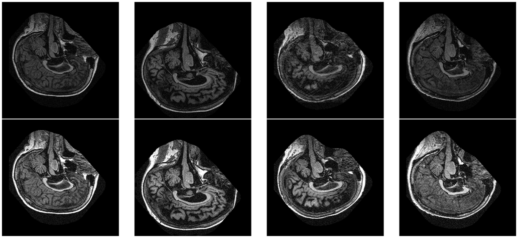
Effect of contrast stretching on the MR images (the top row shows the original images, while the corresponding columns in the second row show the processed images).

These preprocessed images were subjected to segmentation using the improved k-means algorithm. We have improved the state-of-the-art k-means algorithm by selecting centroids in a proper way rather than using random centroids. To the best of our knowledge, all the published work only used manual segmentation of GM, WM and CSF. To extract these individual components, k-means clustering is performed. The performance of the proposed system is evaluated on the OASIS dataset that comprises 128 patients’ data. In the first step, the MR images are preprocessed using contrast stretching. As our aim was to segment out the MR images, high-contrast images were required. Figure 2 shows the results of contrast stretching over a sample image. The top row shows the original images and the corresponding second row shows the processed images.

Figure 3.

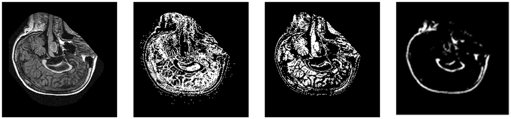
Image segmentation using improved k-means clustering which separates WM, GM and CSF.

Features were extracted from the segmented components of the human brain MRI image. Features incorporating textural, statistical and shape-based information were extracted from those components. Statistical features were extracted such as mean, standard deviation, kurtosis and skewness. GLCM and SURF were extracted as the textural features with HoG as the shape-based features. Graphical representation of textural feature descriptors using GLCM and shape-based features HoG are shown in Figure 4.

Figure 4.

The features extracted from the MR images (the top row shows the HoG features, while the bottom row shows SURF).

Multiclass classification remains an important research problem for AD. The reason for the low accuracy of multiclass classification is the non-identification of discriminative features and the class imbalance problem. Some of the published results are reasonably good, but this problem faces severe class imbalance problem which makes it unreliable. To handle this issue, we have performed resampling with the substitute method on the dataset to produce synthetic data. This enabled us to handle the class imbalance problem in the OASIS dataset. Second, FLDA is used to select the most discriminative features along with reducing the feature vector dimension.

The classification results show a significant achievement of accuracy over the dataset for multiclass classification. Distinguishing the level of dementia is a much more challenging task as compared to the presence and absence of Alzheimer’s in a test subject. Subjects have been classified to detect the level of dementia. Four different classes have been introduced against which subjects are classified to have no dementia, very mild dementia, mild dementia or totally demented. Data samples have been classified over multiple classification algorithms such as SVM and KNN. Data samples belonging to each class are classified using the classification algorithms under the one-versus-all approach. Classification results for each class are averaged giving an overall accuracy of the multiclass classification system. The overall accuracy of all the classification algorithms was recorded, and it seemed that the classification results showed a significant improvement from the techniques discussed in the literature. Results showed that the simple KNN outperformed the SVM by a fine margin. Results calculated over the utilized classification schemes are given in Table 2.

Table 2.

The multiclass classification results for KNN and SVM.

Serial No.	Classification algorithm	Accuracy	Recall	F1-measure
1	KNN	92.7	92.64	92.7
2	SVM	88.21	88.20	88.2

KNN: k-nearest neighbour; SVM: support vector machine.

A comparison is presented in Table 3 with the published results for multiclass classification of AD in The table. Tooba et al. developed an algorithm for multiclass classification using a hybrid feature vector based on textural and shape-based features along with the clinical data. They segmented the image manually and then extracted the features from each segment separately.

Table 3.

Comparison with the existing published work for multiclass classification of Alzheimer’s disease.

Serial No.	Algorithm	Classifier	Dataset	Accuracy (%)
1	Proposed algorithm	KNN	OASIS	92.7
2	MRI + clinical data⁷	SVM	OASIS	79.8
3	MR + hybrid feature⁴	LDA	ADNI	62.7

MRI: magnetic resonance imaging; KNN: k-nearest neighbour; SVM: support vector machine; LDA: linear discriminant analysis.

However, they have not used any technique to handle the class imbalance problem. They were able to achieve 79.8% results for multiclass classification. Another system developed by L Sorenson et al. used textural features along with the thickness of the brain regions as a feature. They were able to produce a 62.7% accuracy over the ADNI dataset. On the other hand, we were able to achieve better accuracy while automatically performing segmentation and handling the class imbalance problem simultaneously.

Conclusion

An efficient approach is used to propose the scheme for the detection of AD at the early stage of disease progression. Contrast-stretched images from the OASIS database are segmented using k-means into segments of GM, WM and CSF. Segmented MR images are used to detect AD using the textural, morphological and shape-based features. GLCM and SURF are used as the textural features, while shape-based features are provided in the form of HoG. The different feature sets are combined forming a hybrid super-feature vector which is reduced by selecting the discriminative subset of features using FLDA. Consequently, three well-known classifiers KNN, SVM and random forest are used to evaluate the proposed methodology using the dataset of OASIS. The mentioned dataset is used to evaluate effectiveness by considering the parameters of accuracy, recall and F-measure. Drawing the comparative analysis with the existing techniques, it is found that the proposed technique outperformed the existing techniques by achieving a 92.7% accuracy, thus becoming one of the benchmark techniques for multiclass classification of AD.

Footnotes

Handling Editor: Arun Sangaiah

Declaration of conflicting interests

The author(s) declared no potential conflicts of interest with respect to the research, authorship, and/or publication of this article.

Funding

The author(s) disclosed receipt of the following financial support for the research, authorship, and/or publication of this article: This study was supported by the research fund from Honam University (2018).

ORCID iD

Ran Baik

References

Ben Ahmed

Mizotin

Benois-Pineau

et al . Alzheimer’s disease diagnosis on structural MR images using circular harmonic functions descriptors on hippocampus and posterior cingulate cortex. Comput Med Imaging Graph 2015; 44: 13–25.

Ben Ahmed

Benois-Pineau

Allard

et al . Classification of Alzheimer’s disease subjects from MRI using hippocampal visual features. Multimed Tools Appl 2015; 74(4): 1249–1266.

Wang

Zhang

Liu

et al . Detection of Alzheimer’s disease by three-dimensional displacement field estimation in structural magnetic resonance imaging. J Alzheimers Dis 2016; 50(1): 233–248.

Sørensen

Igel

Pai

et al . Differential diagnosis of mild cognitive impairment and Alzheimer’s disease using structural MRI cortical thickness, hippocampal shape, hippocampal texture, and volumetry. Neuroimage Clin 2017; 13: 470–482.

Beheshti

Demirel

Farokhian

et al . Structural MRI-based detection of Alzheimer’s disease using feature ranking and classification error. Comput Methods Programs Biomed 2016; 137: 177–193.

Beheshti

Demirel

Feature-ranking-based Alzheimer’s disease classification from structural MRI. Magn Reson Imaging 2016; 34(3): 252–263.

Altaf

Anwar

Gul

et al . Multi-class Alzheimer’s disease classification using image and clinical features. Biomed Signal Proces 2018; 43: 64–74.

Beheshti

Maikusa

Matsuda

et al . Histogram-based feature extraction from individual gray matter similarity-matrix for Alzheimer’s disease classification. J Alzheimers Dis 2017; 55(4): 1571–1582.

Mohanaiah

Sathyanarayana

Guru Kumar

Image texture feature extraction using GLCM approach. Int J Sci Res Publ 2013; 3(5): 1.

10.

Ramaniharan

Manoharan

Swaminathan

Laplace Beltrami eigen value based classification of normal and Alzheimer MR images using parametric and non-parametric classifiers. Expert Syst Appl 2016; 59: 208–216.

11.

Klöppel

Stonnington

Chu

et al . Automatic classification of MR scans in Alzheimer’s disease. Brain 2008; 131(3): 681–689.

12.

Plocharski

Østergaard

LR.

Extraction of sulcal medial surface and classification of Alzheimer’s disease using sulcal features. Comput Methods Programs Biomed 2016; 133: 35–44.

13.

Belleville

Fouquet

Duchesne

et al . Detecting early preclinical Alzheimer’s disease via cognition, neuropsychiatry, and neuroimaging: qualitative review and recommendations for testing. J Alzheimers Dis 2014; 42(Suppl. 4): S375–S382.

14.

Liu

Teverovskiy

Carmichael

et al . Discriminative MR image feature analysis for automatic schizophrenia and Alzheimer’s disease classification. In: Proceedings of 7th international conference on medical image computing and computer-assisted intervention, Saint-Malo, 26–29 September 2004. Berlin; Heidelberg: Springer.

15.

Zhang

Wang

Sui

et al . Multivariate approach for Alzheimer’s disease detection using stationary wavelet entropy and predator-prey particle swarm optimization. J Alzheimer’s Dis 2018; 65(3): 855–869.

16.

Zhang

Wang

Phillips

et al . Three-dimensional eigenbrain for the detection of subjects and brain regions related with Alzheimer’s disease. J Alzheimers Dis 2016; 50(4): 1163–1179.

17.

Lin

C-T

Chuang

C-H

Cao

et al . Forehead EEG in support of future feasible personal healthcare solutions: sleep management, headache prevention, and depression treatment. IEEE Access 2017; 5: 10612–10621.

18.

Lin

C-T

Liu

Y-T

S-L

et al . EEG-based brain-computer interfaces: a novel neurotechnology and computational intelligence method. IEEE Syst Man Cybern Mag 2017; 3(4): 16–26.

19.

Cao

Lin

C-T

Chuang

C-H

et al . Resting-state EEG power and coherence vary between migraine phases. J Headache Pain 2016; 17(1): 102.

20.

Cao

Lin

C-T.

Inherent fuzzy entropy for the improvement of EEG complexity evaluation. IEEE T Fuzzy Syst 2018; 26(2): 1032–1035.

21.

Beheshti

Demirel

Matsuda

Classification of Alzheimer’s disease and prediction of mild cognitive impairment-to-Alzheimer’s conversion from structural magnetic resource imaging using feature ranking and a genetic algorithm. Comput Biol Med 2017; 83: 109–119.

22.

Guerrero

Wolz

Rao

et al . Manifold population modeling as a neuro-imaging biomarker: application to ADNI and ADNI-GO. Neuroimage 2014; 94: 275–286.

23.

Sarraf

DeSouza

Tofighi

DeepAD: Alzheimer’s disease classification via deep convolutional neural networks using MRI and fMRI. BioRxiv. Epub ahead of print 21 August 2016. DOI: 10.1101/070441.

24.

Huang

D-Y

Lin

T-W

W-C.

Automatic multilevel thresholding based on two-stage Otsu’s method with cluster determination by valley estimation. Int J Innov Comput Inform Contr 2011; 7(10): 5631–5644.

25.

Ding

Lin

C-T

Cao

Shared nearest-neighbor quantum game-based attribute reduction with hierarchical coevolutionary spark and its application in consistent segmentation of neonatal cerebral cortical surfaces. IEEE T Neur Net Lear. Epub ahead of print 6 November 2018. DOI: 10.1109/TNNLS.2018.2872974.

26.

Ding

Lin

C-T

Cao

Deep neuro-cognitive co-evolution for fuzzy attribute reduction by quantum leaping PSO with nearest-neighbor memeplexes. IEEE T Cybernetics. Epub ahead of print 22 May 2018. DOI: 10.1109/TCYB.2018.2834390.

27.

Ding

Lin

C-T

Prasad

et al . A layered-coevolution-based attribute-boosted reduction using adaptive quantum-behavior PSO and its consistent segmentation for neonates brain tissue. IEEE T Fuzzy Syst 2018; 26(3): 1177–1191.

28.

Kaur

Choudhary

Comparison of several contrast stretching techniques on acute leukemia images. Int J Eng Innov Tech (IJEIT) 2012; 2: 332–335.

29.

Ishtiaq

Majeed

Maqsood

et al . Improved scalable recommender system. Nucleus 2016; 53(3): 200–207.

30.

Karami

Prasad

Shehata

Image matching using SIFT, SURF, BRIEF and ORB: performance comparison for distorted images. arXiv preprintarXiv:1710.02726, 2017, https://arxiv.org/abs/1710.02726

31.

Kalsoom

Maqsood

Ghazanfar

et al . A dimensionality reduction-based efficient software fault prediction using Fisher linear discriminant analysis (FLDA). J Supercomput 2018; 74: 4568–4602.

32.

Ateeq

Majeed

Anwar

et al . Ensemble-classifiers-assisted detection of cerebral microbleeds in brain MRI. Comput Electr Eng 2018; 69: 768–781.

33.

Darwish

Hassanien

Elhoseny

et al . The impact of the hybrid platform of internet of things and cloud computing on healthcare systems: opportunities, challenges, and open problems. J Amb Intel Hum Comp. Epub ahead of print 15 August 2017. DOI: 10.1007/s12652-017-0659-1.

34.

Shehab

Elhoseny

Muhammad

et al . Secure and robust fragile watermarking scheme for medical images. IEEE Access 2018; 6: 10269–10278.

35.

Elhoseny

Abdelaziz

Salama

et al . A hybrid model of internet of things and cloud computing to manage big data in health services applications. Future Gener Comp Sy 2018; 86: 1383–1394.

36.

Mehmood

Sajjad

Muhammad

et al . An efficient computerized decision support system for the analysis and 3D visualization of brain tumor. Multimed Tools Appl. Epub ahead of print 15 June 2018. DOI: 10.1007/s11042-018-6027-0.

37.

Sajjad

Khan

Jan

et al . Leukocytes classification and segmentation in microscopic blood smear: a resource-aware healthcare service in smart cities. IEEE Access 2017; 5: 3475–3489.

Class imbalance learning–driven Alzheimer’s detection using hybrid features

Abstract

Keywords

Introduction

Related work

The proposed methodology

Image preprocessing

Contrast stretching

Image segmentation

k-Means segmentation

Feature extraction

Statistical features

Textural features

Shape-based features

The class imbalance problem

Feature selection

Classification

Experimentation and results

Dataset

The accuracy assessment

Results and discussion

Conclusion

Footnotes

Declaration of conflicting interests

Funding

ORCID iD

References