
Abstract
Focusing on detecting the illegal behavior of dumping dredged sediments by dredgers at ports, a sensor network composed of two acoustic sources and several passive sensor arrays is proposed in this article. The approach can be divided into two parts: the local sensor decision model and the fusion center algorithm. Local sensors receive signals emitted from the acoustic sources and extract the corresponding Hilbert–Huang marginal spectrum, which is significantly different between the scenario of illegal dumping dredged sediments and the contrary. Local decision is made based on spectrum feature extraction and classification. In regard to the fusion center, a fusion strategy with a scanning window is adopted to make a system-level decision. With a proper window width and the corresponding Bayes optimum threshold, the proposed approach performs well in simulations, in terms of a low system-level false alarm probability and a low system-level miss alarm probability.
Keywords
Introduction
Marine transportation, in its long history, has a close relationship with the maritime countries’ development. As a result, the port, which acts as a hinge linking the ocean and the land, is more and more important. Port is a complicated system composed of many facilities, one of which is called disposal site, that is, waste-dumping zone for dredged sediments. Dredged sediments, which are sediments excavated from the bottom of waterway including ports and estuaries, are expected to be dumped to the disposal site by dredgers. The underwater excavation and dumping process is called dredging. Dredging is important to maintain the depth of waterway. If dredging is performed in a perfunctory manner or not done in time, it will bring hidden safety troubles for the navigation, shipping, and ship berthing.
However, dredgers often dump dredged sediments on the road during their transportation instead of to the prescribed disposal site. Such behavior is harmful and illegal. Therefore, we need a stable and reliable method to detect the misbehavior, viz illegal dumping. Insofar, as it can be ascertained, the related schemes can be classified into two types: ship-equipping and ship-equipping-free. Ship-equipping refers to the approaches depending on installing associated apparatus on board to detect the dumping behavior, for instance, the CCTV video monitoring device 1 and the monitoring recorder for marine wastes dumping. 2 By contraries, ship-equipping-free approaches could work without equipping any devices on dredgers. Thought ship-equipping schemes can achieve better judgments, they would give rise to many problems, for example, ambiguity of liability. Thereby ship-equipping-free detecting has drawn the attention of multiple researchers. The most popular approach is to measure the waterline of dredgers with the starting point: sediments dumping lightens a dredger. Luo et al. 3 advanced a method for automatic detection of ships’ waterline based on the image-processing method, using Canny operators to detect edges and Hough transform to detect the locations of water trace and the waterline after geometric correction. Liu et al. 4 forwarded a texture spectrum method, using K-means clustering algorithm to segment ship waterline images. Gai et al. 5 used a laser rangefinder to get the waterline, but the equipment is expensive, and the method has high requirements for the water turbidity and the measuring cycle period. Hua 6 proposes five dynamic measuring methods to detect the waterline. These methods are little affected by wind and waves. Nevertheless, they have respective limitations: very limited detection range, prohibitive cost of necessary equipment, strict requirements for installation, and so on.
Another way is to detect the presence of flowing sediments below the sea surface. The underlying principle is that flowing sediments will cause the suspended sediment concentration higher than usual. Therefore, we can monitor the suspended sediment concentration, or utilize the impacts of the concentration change to detect the presence of flowing sediments. If a dredger is detected having flowing sediments on its way to the disposal site, it is declared to dump dredged sediments illegally. This involves a subject known as underwater target detection. Unfortunately, the problem abovementioned has rarely been discussed. The detecting targets of most relative literatures are fishes or sea bed sediments,7–10 not the diffusional flowing sediments. Therefore, in order to meet the need of the background, we develop a new approach in the article based on marginal spectrum of Hilbert–Huang Transform (HHT) for local sensors to detect the event.
Furthermore, a network, accompanied by a global fusion approach, is developed to monitor the whole ship channel. Detection fusion has drawn significant attention from academia. Niu and Varshney 11 proposed a counting-rule-based approach which used the total number of detections coming from local sensors as the fusion statistic. A local vote decision fusion approach was introduced by Katenka et al. 12 Applying the principle, whereby the minority is subordinate to the majority, the decision of a local sensor was voted by its entire neighborhood within a fixed distance. Song et al. 13 proposed a scan statistic–based fusion approach, using a scanning window to find the most significant detection cluster in a special part of the data set. In this article, we will show that the fusion strategy with scan statistic is suitable to our network-based application, which is detailed in the following section.
The remainder of the article is organized as follows. Section “Related work” discusses the related work. Section “Detection approach for local sensors” presents our approach of detection for local sensors. Section “Global detection fusion” addresses the data fusion problem of our detection network. Section “Experimental results” presents our simulation results. Section “Conclusion and future work” draws the conclusion and discusses the future work.
Related work
There are several researches on sediment-related issues. The issues can be divided into several types: sediment dredge-and-dump strategies, 14 suspended sediment concentration monitoring, 15 sediment pollution problem, 16 and the ecological effect. 17 And at present, Haimann et al. 18 propose an ecologically oriented integrated monitoring system which consists of several stages, for example, preliminary assessment stage and post-dumpling monitoring stage.
In order to detect suspended sediment concentration, for both Cutroneo et al. 15 and Blanco et al., 16 the dredger needs to be equipped with an acoustic Doppler current profiler (ADCP). ADCP is a kind of equipment which makes use of the Doppler effect of acoustic wave scattered back from particles within the water column to measure water current velocities over a depth range. That is, ADCP emits signal into the water and collects the signal reflected by the particles in the water. Therefore, one can estimate the suspended sediment concentration based on the backscatter intensity.
All the related studies take the detection of the suspended sediment concentration as an indicator to guide the dredgers finishing the dredging operations effectively. The dredgers are assumed to do their duty and follow the instructions well. However, the dredgers in China are employed from third-party companies. And because of the chaos in the management, many dredgers try to find various excuses to remove the monitor facilities equipped on them, and dump dredged sediments on the road during their transportation instead of to the prescribed disposal site to reduce fuel consumption. Therefore, we need a ship-equipping-free approach to detect suspended sediment concentration and take the result as an indicator of whether the illegal dumping happened. Unfortunately, to the best of our knowledge, there is no reference focused on similar application background. Therefore, we strive to develop an effective approach to detect the illegal dumping behavior and take advantage of network structure to extend the detection coverage area.
Detection approach for local sensors
Typically, like Niu and Varshney
11
and Katenka et al.,
12
each sensor obtains an energy reading from the environment. However, the pattern is not applicable in our application, as the suspended sediments would not emit any energy signal. Therefore, we introduce position-fixed acoustic sources (equipped with underwater transducers), and develop a single-input single-output (SISO) detecting model for local sensors (equipped with hydrophones). The detecting signal transmitted by the acoustic sources periodically is composed of two parts: hyperbolic frequency modulated (HFM) signal as synchronization code (denoted by
Model establishment
Denote r(t) as the signal segment received corresponding to s(t) (

that is, we consider a multipath channel, where L is the number of paths decided by the Zielinski N-path model,
19
In the shallow sea,

where

where
The acoustical absorption coefficient

where
Flowing dredged sediments under the sea surface are assumed to exist in forms of particle clouds. Figure 1 is a schematic illustration when a single acoustic ray travels through a particle cloud. Let us take the example of Xiamen Port in China. The concentration of the suspended sediments in the sea at Xiamen Port has consistently kept at a low level less than 0.1%, whereas it will locally exceed 1% in a short time when there is a dredger dumping sediments, which leads

Schematic illustration of the acoustic signal passing through the particle cloud.
The semiempirical formula of

where e is the base of the natural logarithm, A and B are constant with the value 2.03 × 10⁻⁶ and 3.38 × 10⁻⁶, respectively, f is the frequency of the acoustic signal (kHz), d is the depth of the transducer, T is the temperature of the sea surface, we take it as 21.5°C at Xiamen Port, fT is the relaxation frequency with the value
The semiempirical formula of

where C is the volume fraction of the solid particulate;
Parameter calculating formulas for

As shown in Figure 1, we denote

Local sensor node decision
By performing HHT on r(t), we obtain the corresponding Hilbert marginal spectrum. HHT is a time–frequency analysis method advanced in 1998 by Norden E. Huang et al. Compared with the classical signal analysis methods (e.g. the Fourier transform), HHT breaks out the restrains of linearity and stationarity and overcomes the restriction of Heisenberg uncertainty principle.
Denote

where E0 is the energy within the frequency range from 20 to 25 kHz, and

Hilbert marginal spectrums of the signals received under different situations.
Once the feature selection is done, a specific classifier is used to discern the scenario of illegal dumping sediments and the contrary. Thereafter, the local sensor declares its decision accordingly, that is, declares the value 1 when an illegal dumping behavior happened, and declares the value 0 for the opposite case.
Global detection fusion
Optimal detection fusion rule with scan statistic
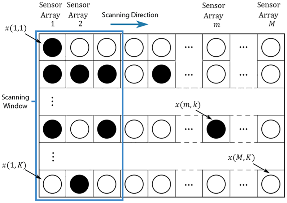
As shown in Figure 3, the sensor network is composed of two acoustic sources and M sensor arrays. Each sensor array contains K passive sensors arranged in the vertical direction. The first

The sensor network is composed of two acoustic sources and M sensor arrays, each of which contains K passive sensors, in order to detect dredgers’ misbehavior of illegal dumping sediments.
Denote the binary data from the kth sensor of sensor array m (i.e. sensor (m,k)) as
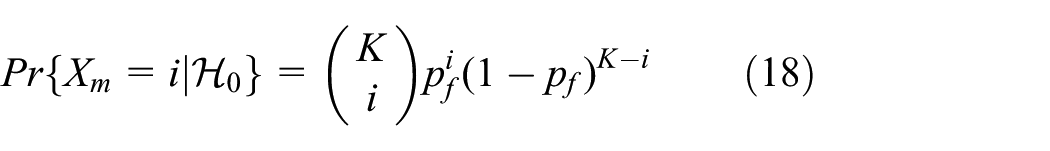
The null hypothesis of no event happens is
If all sensor decisions are counted to get a system-level decision, it is obvious that we can get an extreme low system-level false alarm probability (denoted by
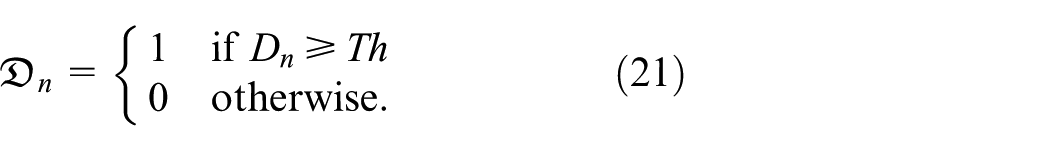
As shown in Figure 4, a counting rule within a scanning window is adopted in this article, using the total number of “1”s wherein as a statistic. Denote the discrete width and height of the window by

where

The maximal scan statistic
where
Data table at the fusion center. x(m, k) or xmk denotes the decision made by the kth sensor of sensor array m, that is, sensor (m, k). The solid circles refer that the corresponding decisions are “1”s.
We call the particular window with the maximal statistic
It is obvious that each sensor may have different false alarm probability and detection probability. In this case,
When

where

where
Note that

where

We assume that
If the fusion center declares
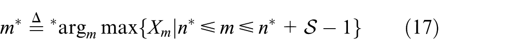
and it indicates that the event happens nearby the geometric plane passing the line which goes through the m*th sensor array and the corresponding acoustic source.
Performance analysis
According to the local detection model described in the previous section, we can get the knowledge of each sensor’s false alarm probability
Under
where

Likewise, the system-level detection probability is calculated as

Because the local decisions made by the sensors under
The equations for calculating
Accordingly, equation (19) is rewritten as

Based on Katenka et al., 12 we arrive at

where

where
Denote the collection of the sensors related to Dn by Ln, that is,
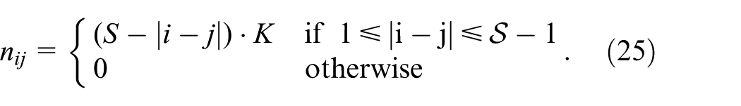
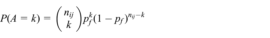
Denote the number of positive decisions made in the intersection by A, the number of positive decisions made in Li but not in Lj by B and the number of positive decisions made in Lj but not in Li by C. Note that A, B, and C are independent. Therefore

where
and

Then the covariance is given by
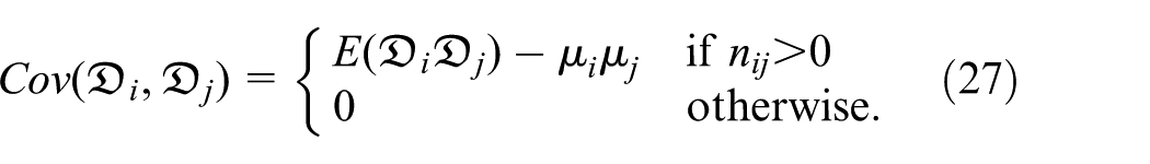
By plugging equation (27) into equation (23), the estimate of
Experimental results
All the simulations are done by MATLAB. The parameters associated with the real environment (e.g. the mean radius of the solid particulate as) are decided according to the practical situations of Xiamen Port.
Local detection
Simulation parameters and performance metrics
The usable frequency range of the transducer is from 20 to 25 kHz, and the code duration is 10 ms. Other simulation parameters are listed in Table 2. The model to simulate the falling process of the dredged sediments is given in another paper,
28
which is needed to decide the value of
Simulation parameters for local detection scheme.

The depth of the navigation channel is set to 16 m.
As it is a binary detection problem (binary hypothesis testing), the metrics should be the detection probability (i.e.
Numerical results
To start with, we discuss the effectiveness and reliability of the feature selection and classification processes. Figures 5–7 have shown that the three features described by equation (8) can be used to discern the scenarios of illegal dumping sediments (yellow box-plots shown in these figures) and the contrary (green box-plots shown in these figures). The values of each box-plot are obtained from the results over 103 simulation runs. As shown in Figure 5, the main value range of

The peak energy values between the scenarios of illegal dumping sediments and the contrary (marked as the label “NoDump”). Each box-plot is obtained from the results over 103 simulation runs: (a) the impact of different dumping volumes. The dumping location is110 m far away from the signal emitting end. (b) The impact of different dumping locations. The volume of the dredged sediments dumped is 50 m 3 . The dumping location is the distance from the signal-emitting end.

The ratios between 3 dB bandwidth and 50 kHz under the scenarios of illegal dumping sediments and the contrary (marked as the label “NoDump”). Each box-plot is obtained from the results over 103 simulation runs: (a) the impact of different dumping volumes. The dumping location is110 m far away from the signal emitting end. (b) The impact of different dumping locations. The volume of the dredged sediments dumped is 50 m 3 . The dumping location is the distance from the signal-emitting end.

The ratio between the energy within the frequency range from 20 to 25 kHz and total energy under the scenarios of illegal dumping sediments and the contrary (marked as the label “NoDump”). Each box-plot is obtained from the results over 103 simulation runs: (a) the impact of different dumping volumes. The dumping location is110 m far away from the signal emitting end. (b) The impact of different dumping locations. The volume of the dredged sediments dumped is 50 m 3 . The dumping location is the distance from the signal-emitting end.
However, any one of the features would fail to discern the two kinds of scenarios with high accuracy, as their value ranges are not entirely different. Especially when the extreme outliers are generated, miscarriage of justices would be made. Therefore, the following classifiers are tested using all of the features to see which one is preferred: LibSVM, K nearest neighbors (KNN) classifier, Naive Bayes classifier and discriminant analysis classifier.
As shown in Figures 5–7, Ep is much bigger than the other two features, thereby Ep should be processed first. Because the highest value of Ep is not bigger than 20, so we use Ep/20 instead of Ep as a classification feature.
A total of 6900 simulation results under 14 different conditions, that is, no dredged sediments dumped (3000 data) and 50 m 3 dredged sediments dumped at 13 different distances from the emitting end (13 × 300 data), are used for training. Another 23,100 simulation results under 25 different conditions, that is, no dredged sediments dumped (3000 data), 50 m 3 dredged sediments dumped at 13 different distances from the emitting end (13 × 700 data), and 11 different volumes of dredged sediments dumped at the distance 110 m far away from the emitting end (11 × 1000 data), are used for predicting.
Classification results are shown in Figure 8(a). The recognition success rates are judged by a single detecting code. Unfortunately, the false alarm probabilities (i.e. the detection probabilities for the scenario of no dredged sediments dumped in the figure) are too high, which are above 10% on the whole. It is worth noting that, as mentioned before, there are several (here we choose three) evenly spaced detecting codes in a detecting signal. So the judgment should be made by the three detecting codes together. When the minority is subordinate to the majority, the recognition success rates judged by a complete detecting signal are shown in Figure 8(b).

The recognition success rates of the local sensor detection approach proposed: (a) judged by a single detecting code and (b) judged by a complete detecting signal (three detecting codes).
As depicted in Figure 8(b), false alarm probabilities
Global fusion
We hope the system-level detection probability
As indicated in Figure 8, local sensors can achieve high

The relationship between
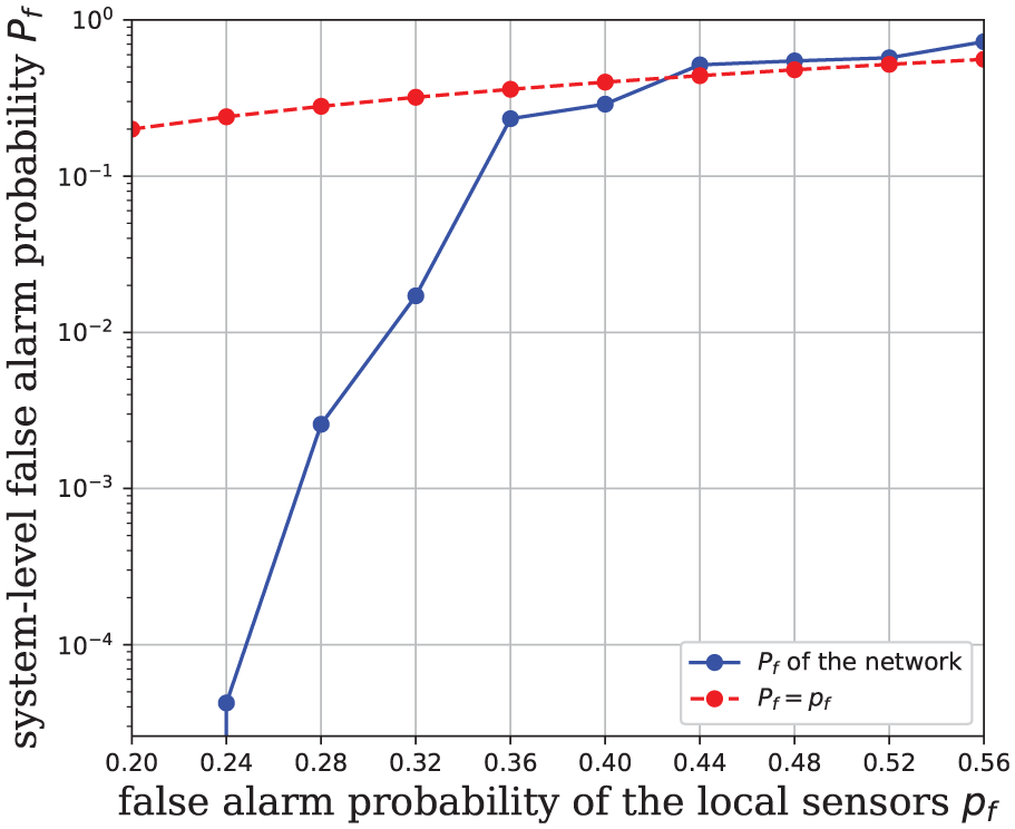
The relationship between the system-level false alarm probability
It is clear from Figure 11 that the performance depends on the threshold Th. Double y axes are also adopted here. We notice that the Bayes threshold is optimal.

The relationship between
Conclusion and future work
This article seeks an adequate solution to the problem of detecting dredgers’ illegal behavior of dumping dredged sediments. The solution is composed of a local sensor detection approach and a fusion strategy. In the local sensor part, an acoustic signal propagation model for sediments dumping channel is built first, and then an effective detection approach is presented. The local false alarm probabilities and miss alarm probabilities are both less than 5% for all candidate classifiers, which could be as low as about 4% and 3%, respectively for LibSVM. When the lowest false alarm probability is preferred, Naive Bayes classifier is a better choice with about 2% false alarm probability.
At the fusion center, a scan statistic is used to fuse the decisions made by the local sensors, by which we can make a tradeoff between the system-level false alarm probability
In the future, to offer a more flexible detection network, the sensors will be deployed on buoys or autonomous underwater vehicles, no longer fixed on the shore. Therefore, it is essential to make the sensors be able to plan their paths, in order to minimize the redundant coverage overlap, that is, maximize the overall detection area. Furthermore, when a dredger is working, the sensors are expected to follow the dredger. Once the algorithms are done, the deployments in the real environment (for example, a harbor) may be performed.
Footnotes
Handling Editor: Florentino Fdez-Riverola
Declaration of conflicting interests
The author(s) declared no potential conflicts of interest with respect to the research, authorship, and/or publication of this article.
Funding
The author(s) disclosed receipt of the following financial support for the research, authorship, and/or publication of this article: This work was supported by the National Natural Science Foundation of China (grant nos: 61471308, 61571377, and 61771412) and the Fundamental Research Funds for the Central Universities (grant no.: 20720180068).