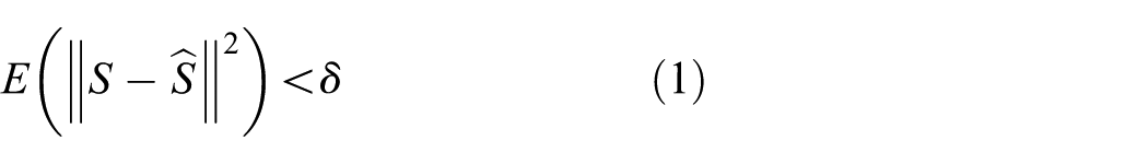
Sage Journals: Discover world-class research

Abstract

Energy efficiency is one of the most crucial concerns for WSNs, and almost all researches assume that the process for data transmission consumes more energy than that of data collection. However, a few sophisticated collection processes of sensory data will consume much more energy than traditional transmission processes such as image and video acquisitions. Given this hypothesis, this article proposed an adaptive sampling algorithm based on temporal and spatial correlation of sensory data for clustered WSNs. First, according to spatial correlations between sensor nodes, a distributed clustering mechanism based on data gradient and residual energy level is proposed, and the whole network is divided into several independent clusters. Afterwards, each cluster head maintains an autoregressive prediction model for sensory data, which is derived from historical data in the temporal domain. With that, each cluster head has the ability of self-adjusting temporal sampling intervals within each cluster. Consequently, redundant data transmission is reduced by adjusting temporal sampling frequency while ensuring desired prediction accuracy. Finally, several distinct sampler collection sets are selected within each cluster following intra-cluster correlation matrix, and only one sampler collection needs to be activated at each round time. Sensory data of non-sampler can be substituted by those of sampler due to strong spatial correlation between them. Simulation results demonstrate the performance benefits of proposed algorithm.

Keywords

Wireless sensor networks adaptive sampling prediction model temporal and spatial correlation energy efficient

Introduction

Due to inherent advantages to monitor region of interest (ROI) in a fully distributed manner, wireless sensor networks (WSNs) have drawn considerable research interests and academic attentions in recent years.^1,2 WSNs consist of a large number of self-organizing sensor nodes which are deployed in interesting or unattainable areas to acquire environmental information. With the advancements in system-on-chip (SOC) miniaturization and integration, it is possible to deploy abundant sensor nodes for practical applications^3,4 Generally, each sensor node in WSNs collects raw sensory data periodically and then transmits to the sink node through wireless multi-hop communication for further analysis. However, this approach will result in excessive communication and energy consumption.

Due to energy-constrained characteristic of WSNs, in recent years, many energy management mechanisms have been proposed to reduce power consumption in the literature. Most researches suppose that energy consumption for data acquisition and processing is significantly lower than that for communication. Therefore, traditional researches focus on conserving energy as much as possible by reducing transmission capacity. Unfortunately, this assumption is not always held in a number of practical applications because acquisition time is typically longer than transmission time. Moreover, some acquisition processes are very sophisticated such as video and image encoding in wireless multimedia sensor networks. Consequently, adaptive sampling mechanism⁵ is regarded as a promising method to improve energy efficiency in recent years, which focuses on reducing the amount of sensory data through self-adaptive sampling method. In addition, sensory data in WSNs usually have spatial correlation (due to geographical closeness of sensor nodes) and temporal correlation (due to smooth variations of signals in real world). Therefore, we investigated one hybrid adaptive sampling algorithm based on spatiotemporal correlation (ASbST in short) to conserve restricted energy.

The main idea of this article is to schedule sensor nodes by activating necessary and optimal sensor nodes with constraints of desired prediction accuracy. In this article, we activate more sensor nodes in data change non-smoothing regions and fewer sensor nodes in data change smoothing regions, thus guaranteeing data collection accuracy as well as reducing energy consumption.⁶ In addition, sampling frequency in the temporal domain of each collection set is regulated by updated rule self-adaptively. With the proposed adaptive and optimal sampling algorithm ASbST, fewer sensor nodes are activated at the same time; meanwhile, the average sampling frequency is reduced. As a result, sensory data necessary for delivery are reduced so as to achieve significant energy conservation.

The rest of this article is organized as follows. Section “Related works” presents an overview in the area of adaptive data gathering. Section “Adaptive sampling for clustered WSNs” illustrates an analytical model and the overall principle of proposed adaptive sampling algorithm for clustered WSNs, and several crucial components of the proposed ASbST algorithm are described in detail from sections “Clusters construction” to “Autoregressive moving average (ARMA)-based predictive model at cluster head (CH).” Simulation and performance evaluation are presented in section “Simulations and analysis.” Finally, section “Conclusion” concludes this article.

Related works

Energy consumption is the most important research issue in WSNs. However, most researches focus on new methods for energy-efficient transmission, and only a few researchers are investigating energy effective adaptive sampling mechanisms. Energy-efficient transmission problem for WSNs has been investigated with mathematical optimization method in literature.⁷ Generally, adaptive sampling mechanisms can be divided into two categories:⁸ adaptive spatial sampling (ASS) algorithms and adaptive temporal sampling (ATS) algorithms. ASS algorithms ensure sampling accuracy using spatial region–based self-adjusting, wake-up/sleep states scheduling, and so on. ATS algorithms ensure sampling accuracy using sampling frequency self-adjusting, online signal tendency estimation, and so on. Figure 1 shows the categories of current adaptive sampling algorithms, which are concluded from a lot of existing literature.

Figure 1.

Sampling strategy categories.

It is well known that WSNs prefer to sample more than requirement, thus resulting in significant spatial and temporal correlations.⁹ Temporal correlation is used in an adaptive sampling algorithm named as adaptive sampling approach (ASAP) to minimize energy consumption of sensor nodes.¹⁰ The main idea of ASAP is to use a dynamically changing subset of nodes as samplers so that sensory readings of sampler nodes are directly collected, whereas sensory data of non-sampler nodes are predicted through designed probabilistic model. Alippi et al.¹¹ propose an adaptive sampling algorithm that estimates online optimal sampling frequencies for sensor nodes and apply it into snow-monitoring applications. Santos et al.¹² present a technique that applies adaptive automata mechanism, and the possibility of sensor networks dynamically vary the interval (time) between a data logging and other, so as to reduce data sampling intervals. Zheng et al.¹³ discuss how to perform energy-efficient sensory data sampling with compressive sensing technology. Our previous work¹⁴ proposes a sample frequency–based adaptive sampling algorithm, where the sampling frequency of each cluster was determined by CH following the multiplicative increase additive decrease (MIAD) rule dynamically. Szczytowski et al.¹⁵ identify the regions of oversampling or undersampling and propose a Voronoi-based ASS (ASample) solution. As a result, it removes unnecessary samples from regions of oversampling and generates additional new sampling locations in the undersampling regions to fulfill specified accuracy requirements. Deligiannakis et al.¹⁶ describe an self-based regression (SBR) algorithm for compressing multi-valued feeds containing historical data from each sensor node. The key to their technique is the base signal—a series of values extracted from real measurements used to provide piece-wise approximation of the measurements. Moreover, they further explain how it can be adapted to exploit correlations among measurements operated on single node/multiple nodes. JB Li and JZ Li¹⁷ propose a method to select some specific sensor nodes among the sensor nodes with stronger spatial correlations, thus reducing the data redundancy. However, this method does not consider the adjustment of the sampling frequency in time domain. Mukhopadhyay et al.¹⁸ propose a data error correction method based on prediction model established in the time domain for WSNs to improve the reliability of sensory data. JZ Li and colleagues.^19,20 focus on designing physical world aware data acquisition algorithms to support O(ε)-approximation to the physical world for any ε and then propose two physical world aware data acquisition algorithms to reconstruct the physical world. Our previous work²¹ proposes a novel coverage ratio index in consideration of the spatial domain and temporal domain as well as a novel coverage sampling technology based on spatial–temporal joint union for WSNs. Most of the above researches are concentrating on adaptive sampling either in the time domain or in the spatial domain, and there are no relevant studies to take these factors into account.

This article aims at designing ATS algorithm combining self-adjusting frequency sampling and ASS and proposes a novel adaptive sampling algorithm based on temporal and spatial correlations of WSNs. To the best of our knowledge, this is the first spatiotemporal correlations–based adaptive sampling algorithm for clustered WSNs. By optimizing sampling frequency and sampling node sets of different clusters adaptively in a distributed manner, the average sampling frequency and number of sampling nodes will decrease so as to decrease energy consumption of whole WSNs. In addition, the proposed algorithm of this article can guarantee sensory data’s sampling accuracy at the same time.

Adaptive sampling for clustered WSNs

System model and overview

In this section, we describe the investigated clustered WSNs model and introduce basic concepts through an overview of adaptive sampling based on temporal and spatial correlation. In our clustered WSNs, a large number of energy-constrained sensor nodes assigned with unique IDs are employed randomly in a rectangle area. Therefore, the network topology of WSNs to be discussed can be represented by an undirected simple graph $G = (V, E)$ in the plane, where $V$ denotes the set of nodes and $E$ the set of edge links of WSNs. The power needed to support a link uv is assumed to be $‖ uv ‖^{π}$ , where $‖ uv ‖$ denotes the Euclidean distance between sensor nodes u and v and $π$ a real constant between 2 and 5 depending on the wireless transmission environment.²² Table 1 shows some notations necessary for this article.

Table 1.

Notations.

Notation	Meaning
$G = (V, E)$	Undirected graph of clustered WSNs
$V$	Collection set of sensor nodes
$E$	Collection set of edge links
$N_{i}$	The ith sensor node
$\| N_{i} \|$	Neighbors’ number of ith sensor node
$p$	Percentage value of cluster head
$r$	Sampling completed set (SCS) granularity
$E_{i}$	Residual energy of ith sensor node
$T h_{min}$	Minimal sampling frequency
$T h_{max}$	Maximal sampling frequency
$θ_{MRE}$	Threshold value of average relative error
$f_{0}$	Initial sampling frequency
$f_{i}$	Current sampling frequency
$α$	Multiplicative increasing factor of samplingfrequency
$β$	Additive decreasing factor of sampling frequency
$M$	Step value of sampling frequency
$T_{s}$	Regular sampling interval
W	Window size of prediction model

MRE: Mean Relative Error.

In addition, we assume that there is a higher node density in our clustered WSNs. Hence, the practical spatial data correlation model described in Lotfinezhad and Liang²³ can be introduced. Let $S$ be a vector of $n$ measured samples collected by $n$ sensor nodes, and $\hat{S}$ be a representation of $S$ . For the purpose of illustration, $S$ is denoted as a spatially correlated random Gaussian vector. In addition, $d (S, \hat{S})$ denotes the distortion rate measurement between $S$ and $\hat{S}$ , which is defined with mean square error (MSE) $d (S, \hat{S}) = ‖ S - \hat{S} ‖^{2}$ . The mean value $d (S, \hat{S})$ is constrained by certain threshold $δ$

E ({‖ S - \hat{S} ‖}^{2}) < δ

(1)

Due to the strong correlations of sensory data in WSNs, we propose a model-based adaptive sampling mechanism for clustered WSNs considering temporal and spatial correlations together. The proposed adaptive sampling algorithm ASbST comprises several components: (1) sensing data driven clustering algorithm. With this algorithm, sensor nodes, similar to each other in terms of their observed sensory data, should be clustered into one group. Furthermore, sensor nodes will join in its nearest CH to be cluster members, thus taking advantage of the spatial correlation measured with Euclidean distance for simplicity. (2) ATS algorithm. Each CH builds a prediction model with historical data within its cluster. Afterwards, it uses predicted value from estimated prediction model to substitute that of non-sampling nodes, thus decreasing sampling frequency, which is shown in Figure 2. The online intra-cluster prediction framework of each CH is described in Figure 3. It establishes and maintains a prediction model by feature extraction from historical data. (3) ASS algorithm. Cluster members are further divided into a few sub-clusters, and only one sensor node with most residual energy in each sub-cluster will be selected to be one member of sampling completed set (SCS). The CH uses sensory reading from its cluster members to abstract the spatial and temporal correlations of sensory data. Then, each cluster is partitioned into some sub-clusters, with the basis of principle that cluster members whose sensory data are highly correlated are divided into the same sub-cluster. As a result, only sensor nodes in SCS of each cluster serve as samplers, and the others belong to non-samplers in order to conserve nodes’ energy.

Figure 2.

Temporal prediction model diagram.

Figure 3.

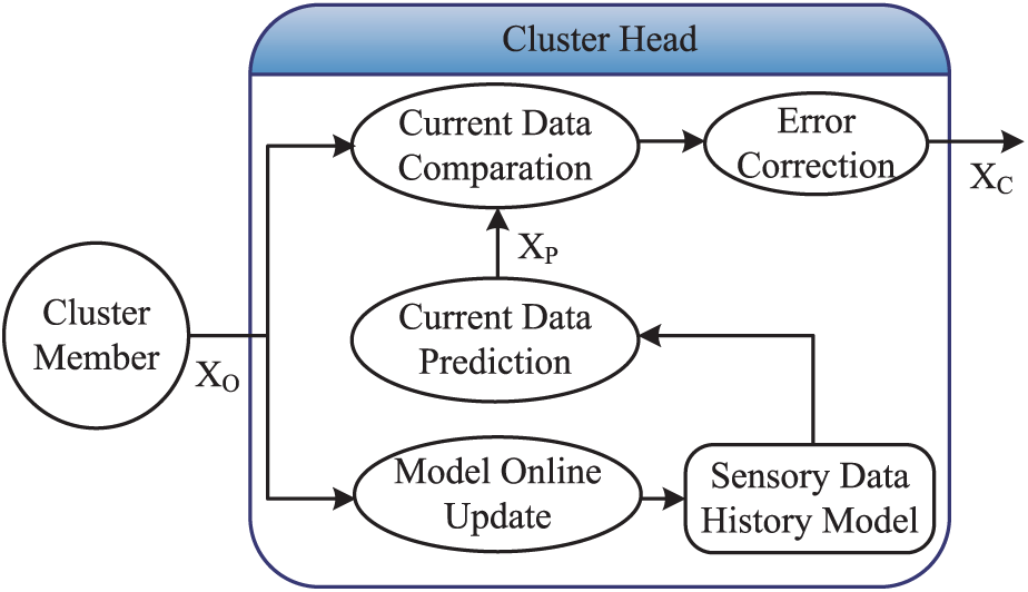
Online intra-cluster prediction framework.

Moreover, in this article, we use network topology and sensory data derived from Intel’s laboratory in Berkeley University²⁴ with 54 sensor nodes deployed in the Lab.

Adaptive sampling in the temporal domain

Figure 4 shows the origin principle of proposed adaptive sampling algorithm in the temporal domain. There is a specific signal whose amplitude is shifting with time sequence. Obviously, oversampling denotes that the actual sampling frequency is much higher than necessary sampling rate, and undersampling shows that actual sampling frequency is much lower than necessary sampling rate. It is a promising research topic to minimize real-time sampling frequency as much as possible while satisfying desired prediction precision. However, it is very hard to acquire appropriate sampling rate because signal frequency is often unknown in advance.

Figure 4.

Nyquist-based fixed sampling, oversampling, and undersampling: (a) fixed sampling rate, (b) oversampling rate, and (c) undersampling rate.

In the work, well-designed ATS strategy is operated in each cluster, and the intra-cluster sampling frequency is determined by each CH. When the deviation value between sampled data and predicted data exceeds a preset threshold, CH will increase intra-cluster sampling frequency; otherwise, CH will decrease intra-cluster sampling frequency. In other words, the intra-cluster sampling frequency can be increased to ensure the quality of sampled data with high dynamic nature of sensory data. Otherwise, the intra-cluster sampling frequency will decrease with low dynamic nature of sensory data, so as to reduce data redundancy. Finally, the balance of energy efficiency and data gathering quality can be achieved together through this method.

Adaptive sampling in the spatial domain

At first, we define two new concepts: oversampling region (the case with much more awaking sensor nodes than necessary) and undersampling region (the case with fewer awaking sensor nodes than necessary). Sensor nodes are partitioned into different clusters according to data gradient metric between sensor nodes in spatial domain. Therefore, the proposed ASS scheme will operate on each cluster in a fully distributed manner. The main principle of adaptive sampling algorithm in spatial domain is to reduce the number of awaking nodes with AR prediction model, which is maintained and updated by each CH. In addition, cluster members of each cluster are further divided into a few sub-clusters based on the historical model of sensory data. The proposed ASS approach is explained with an example (see Figure 5). Seven sensor nodes with ID 1 to 7 in the square ROIs can be divided into two independent sub-clusters named as SCS: {node 1, node 2, node 3, and node 4} and {node 5, node 6, and node7}. Either of them can cover the whole square ROI. In order to conserve energy, only these sensor nodes (named as samplers) in either SCS are awake; meanwhile, sensor nodes in another SCS enter sleeping status, which are named as non-samplers.

Figure 5.

Oversampling spatial region.

Clusters’ construction

The goal of sensing-aware clustering algorithm proposed in this article aims at forming a hierarchical network framework to facilitate adaptive sampling and achieve the optimization objective of energy saving awareness and data gradient awareness. In the first phase, we propose a distributed clustering algorithm to establish one-hop clusters, where CHs are elected in a fully distributed fashion. Each sensor node is elected to be CH randomly with probability $ω_{i}$ , which is defined as

ω_{i} = p \times \frac{E (i) \times | N_{i} |}{\sum_{j \in N_{i}} E (j)}

(2)

where $E (i)$ and $E (j)$ denote the residual energy of sensor node i and j, respectively; $| N_{i} |$ denotes its one-hop nodes’ degree including itself, and $p \in (0, 1]$ is the percent value of CHs. The first system-wide parameter $p$ defines the probability value to be CH with its practical value within the range (0, 0.2]. It is obvious that the defined probability formula has a positive correlation with node’s residual energy. More specially, sensor nodes with more residual energy within all neighbor nodes should be chosen to be CHs with higher probability, thus implementing the principle of maximum residual energy first.

Subsequently, CHs broadcast CH notification messages to their one-hop neighbor nodes after CHs election process. Those cluster members (CMs) that received CH notification messages will make a decision about which CH to join in. It is called as minimal data gradient principle. The details of minimal data gradient principle are illustrated as shown in Figure 6, and there are four CHs locating in the one-hop region of CM_i. The minimal data gradient selection algorithm is described in equations (3) and (4). The CM_i will select the CH with minimal gradient value as its CH, for example, if $\partial f / \partial l_{3} |_{C M_{i}}$ is the minimum, CM_i will join in cluster with CH₃ as its CH

C H = {C H_{j} | \frac{\partial f}{\partial l_{j}} |_{C M_{i}} = \min {\frac{\partial f}{\partial l_{1}} |_{C M_{i}}, \frac{\partial f}{\partial l_{2}} |_{C M_{i}}, \frac{\partial f}{\partial l_{3}} |_{C M_{i}}, \frac{\partial f}{\partial l_{4}} |_{C M_{i}}}}

(3)

{\begin{matrix} \frac{\partial f}{\partial l_{1}} |_{C M_{i}} = \frac{| E_{C M_{i}} - E_{C H_{1}} |}{d (C M_{i}, C H_{1})} \\ \frac{\partial f}{\partial l_{2}} |_{C M_{i}} = \frac{| E_{C M_{i}} - E_{C H_{2}} |}{d (C M_{i}, C H_{2})} \\ \frac{\partial f}{\partial l_{3}} |_{C M_{i}} = \frac{| E_{C M_{i}} - E_{C H_{3}} |}{d (C M_{i}, C H_{3})} \\ \frac{\partial f}{\partial l_{4}} |_{C M_{i}} = \frac{| E_{C M_{i}} - E_{C H_{4}} |}{d (C M_{i}, C H_{4})} \end{matrix}

(4)

where $E_{C M_{i}}$ and $E_{C H_{j}}$ denote the acquired mean value at CM_i and CH_j, respectively; $d (C M_{i}, C H_{j})$ denotes the Euclidean distance between CM_i and CH_j; and $(\partial f / \partial l_{j}) |_{C M_{i}}$ is the gradient value from CM_i to CH_j.

Figure 6.

Minimal data gradient principle.

After clusters construction phase, sensor nodes are divided into two categories: one particular sensor node is elected as CH responsible for data aggregation and the other sensor nodes as cluster members (CMs) responsible for data acquisition. 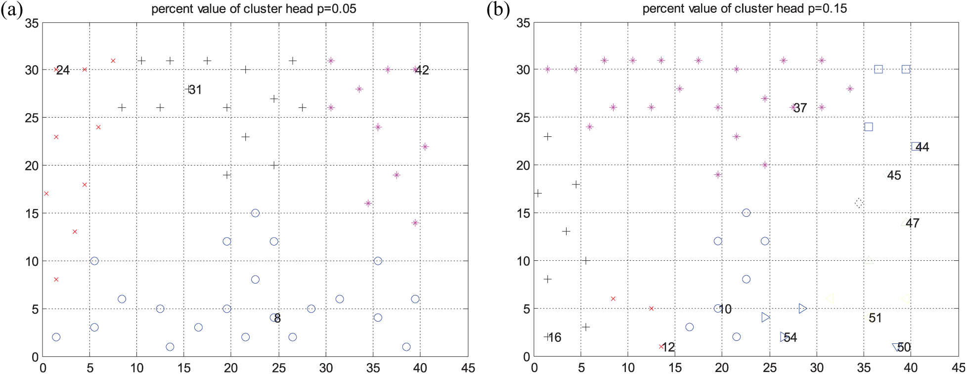The detailed sensing-aware clustering algorithm is illustrated in our previous work.²⁵ Figure 7 demonstrates the clustering results of different CH percent ( $p = 0.05$ and $p = 0.15$ ). In Figure 7, different clustering nodes are labeled with different colors and shapes, and sensor nodes with sign number for each cluster represent CHs.

Figure 7.

Clustering results of different cluster head percent: (a) CH percent (p = 0.05) and (b) CH percent (p = 0.15).

ATS

Following the most famous Nyquist law in signal processing field, if the highest frequency F_max of signal is given, the minimum sampling frequency F_N is more than twice the highest frequency, thus guaranteeing signal reconstruction. In particular, it is common to pick a sampling frequency three to five times higher than the highest frequency of signal, that is, F_N = cF_max, where c = 3–5.²⁶ Unfortunately, highest signal frequency is not available in advance for most applications. Moreover, it will change over time in a non-stationary process. Consequently, the sampling frequency has to vary adaptively with signal variation tendency. For large-scale WSNs with many clusters, signal variation tendencies of different clusters are different, so signal sampling rate ought to adjust subsequently within different clusters.

This research holds the following assumptions: (1) the sensory data of WSNs in the temporal sequence are typically continuous and stable in many practical scenarios and (2) there are some data errors because of unreliable wireless communication, failure of sensor nodes, and so on. Based on the above two hypotheses, more collected sensory data do not mean more accurate results. Moreover, the actual sampling frequency is universally high in the time domain for many applications. For example, it is obvious that historical temperature values of Sensor No. 1 between 1 March and 6 March have strong similarity (as shown in Figure 8), defined as temporal correlations.

Figure 8.

Temporal correlations of different days.

Unfortunately, it is impossible for accurate estimation of signal highest frequency in advance, so we propose an intra-cluster sampling frequency self-adjusting method. Each CH establishes one second-order AR prediction model based on historical data of its cluster members. After that, estimated value is used instead of sampling data which are calculated by AR prediction model. The self-adapting sampling frequency adjustment scheme is described as in the following: the intra-cluster sampling frequency will increase additively by a certain step value when the sampling error is less than the preset threshold; otherwise, the intra-cluster sampling frequency will be reduced to its half value. Figure 9 shows the detailed process of the proposed algorithm. In the each iteration process, each CH broadcasts a certain sampling frequency to its CMs, which is determined by current sampling accuracy. If current sampling error is larger than the default threshold $θ_{MRE}$ , the sampling frequency will increase as $f_{i} = α \times f_{i}$ . The additive decreasing step value $β$ is a fraction of M difference between maximal threshold value and minimal threshold value. On the contrary, if the current sampling error is lower than the threshold value $θ_{MRE}$ , the sampling frequency will decrease as $f_{i} = f_{i} - β$ . Therefore, the sampling frequency self-adapting algorithm complies with the principle that obeys MIAD rule.

Figure 9.

Pseudo-code for adjustment of intra-cluster sampling frequency.

The distributed characteristic of sampling frequency self-adjusting strategy is that different sampling frequency regulation processes are operated on different clusters at the same time. Therefore, the proposed algorithm is appropriate even for large-scale WSNs. The uniform initial sampling frequency of each cluster is determined by the sink node. Moreover, it is same for the minimal sampling frequency $T h_{min}$ and maximal sampling frequency $T h_{max}$ of each cluster, respectively. The mean relative error $(MRE)$ provides a metric of sampling accuracy, which is defined as

MRE = \sqrt{\frac{1}{W} \sum_{i = 1}^{W} {(\frac{X_{i} - \tilde{X_{i}}}{\tilde{X_{i}}})}^{2}}

(5)

where $X_{i}$ denotes the ith collected value in the original data sequence, $\tilde{X_{i}}$ denotes the ith predicted value by CH, and $W$ denotes the window size of samples in the original data sequence.

ASS

The most prominent assumption of the work is that those sensor nodes that are closer to each other will have stronger correlation. For example, Figure 10 shows the data variation tendencies of Sensor Nos 1, 2, 16, and 17 in Intel’s laboratory. It is obvious that the variation tendency of Sensor Nos 1 and 2 is much more similar than that of Sensor Nos 1 and 16. Specially, it is obvious that the sensory data of Sensor No. 17 has many errors because of transmission or acquisition errors. There are two crucial components of the proposed ASS approach. The first one is to facilitate the classification of sensor nodes to serve as distinct sampler, and the other is named as optimized scheduling for sampler and non-sampler.

Figure 10.

Spatial correlations of neighbor sensor nodes: (a) sensory data of Sensor No. 1, (b) sensory data of Sensor No. 2, (c) sensory data of Sensor No. 16, and (d) sensory data of Sensor No. 17.

The most important phase is to construct several distinct sampler collections within each cluster. The cluster formation described in section “Clusters construction” complies with two metrics: sensor nodes similar to each other in terms of sensory data should be clustered together and sensor nodes close to each other should be clustered together. As we know, higher correlations among sensor nodes within a cluster typically lead to higher sampling accuracy. However, this will lead to much lower efficiency of energy at the same time. The principle of proposed idea is to divide cluster members into several sub-clusters, and only one of sensor nodes in each sub-cluster is awake within its sub-cluster. It is supposed that the spatial region of WSNs is almost oversampling with ROI covered by at least two distinct collections. Therefore, our goal of further dividing sensor nodes into sub-clusters is to facilitate the selection of SCS. For example, in Figure 11, one cluster is divided into three sub-clusters (Sub-cluster A, Sub-cluster B, and Sub-cluster C), and Sensor Nos 1, 7, and 5 are selected from each sub-cluster to form an SCS. Once SCS is determined within one cluster, only SCS nodes need to wake up to be sampler and other sensor nodes transform to sleep mode so as to conserve energy. Moreover, sensory data of sleeping sensor nodes can be estimated at each CH using AR prediction model.

Figure 11.

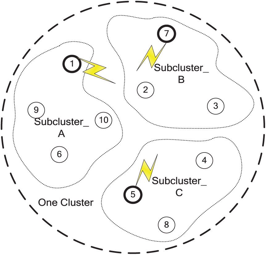
Example of sampling completed sets.

The above three sub-clusters are elected with such optimal metric. First of all, we create a correlation matrix for each twin collection i and collection j. For any two nodes u and v in the collection, $C_{ij}$ is equal to the correlation between series $D_{u}$ and $D_{v}$ . Formally

C_{ij} = | \frac{[D_{u} - E (D_{u})] \times {[D_{v} - E (D_{v})]}^{T}}{L \times \sqrt{Var (D_{u})} \times \sqrt{Var (D_{v})}} | \in [0, 1]

(6)

where $L$ denotes the length of data series, symbol T denotes the matrix transpose. Hence, $C_{ij} = 1$ implies that two series are strongly correlated, while $C_{ij} = 0$ implies that two series are not correlated. Each CH analyzes sampled sensory data from its cluster members to capture the temporal and spatial correlations using the above correlation matrix. The derived sub-clusters are non-overlap, and each one can cover the whole ROI. In conclusion, the objective of sub-cluster collection selection is defined as the optimization problem in Figure 12, thus leading to higher energy efficiency while guaranteeing sampling accuracy. In fact, we introduce agglomerative clustering²⁷ to partition sub-clusters where the above defined correlation value is used as distance metric.

Figure 12.

Optimization objective to select sampling collection sets.

The SCS granularity $r$ is defined as the number of the sub-clusters in each cluster. Intuitively, larger $r$ may decrease the predictive performance because it will result in larger sub-cluster with potentially lower correlations among its cluster members. However, too smaller $r$ may decrease the predictive performance since the opportunity to exploit the spatial correlations will be missed. In Figure 13, the whole WSNs is divided into three clusters (sensor nodes with same color belong to one cluster), and each cluster is divided into two $(r = 2)$ or three $(r = 3)$ distinct sub-clusters (sensor nodes with same shape in the same cluster belong to one sub-cluster).

Figure 13.

Sub-clustering results with different SCS granularity $r$ .

Once optimal SCS are determined in each round, sensor node with maximal residual energy within each sub-cluster is selected to be one member of SCS. As a result, sensor nodes are divided into sampler and non-sampler. Only the former needs to transmit the required data to the sink node instead of the latter. The values of non-sampler nodes will be predicted at CH by prediction model constructed with historical data.

ARMA-based predictive model at CH

The remaining problem is to calculate the previously defined sampling accuracy metric derived at each CH. The famous autoregressive and moving average (ARMA) model captures the autocorrelation in a data set by expressing the prediction as a linear combination of previous samples. This article adopts a smaller amount of calculation of linear AR model²⁸ to sample prediction model at each CH. Meanwhile, it uses the recursive least squares (LS) estimation methods for parameter estimation, which is described as follows

X_{p} [n] = \sum_{i = 1}^{W} a_{i} [n] \cdot X [n - i]

(7)

e [n] = X [n] - X_{p} [n]

(8)

where $X_{p} [n]$ denotes predicted value, $X [n]$ the actual sampled value, $e [n]$ the predictive error, and $a_{i} [n]$ different order coefficients of AR model. The applied model is characterized in terms of model order $W$ , which defines the size of AR model. It is well known that the model consists of estimation of coefficients $a_{i} [n]$ , for which this work uses recursive least square (LS) estimation because linear prediction functions can be computed efficiently.

Considering such requirements as prediction accuracy and operation speed, two-order AR prediction model is introduced. Thus, the predictive value can be reconstructed by each CH with historical data

{\hat{X}}_{i + 1} = k_{1} (X_{i} - \bar{X}) + k_{2} (X_{i - 1} - \bar{X}) + e_{i + 1}

(9)

where $k_{1}$ and $k_{2}$ denote two coefficients for two-order AR model, respectively; $e_{i + 1}$ denotes predictive error; and $\bar{X}$ the average value of W historical data. Moreover, two coefficients $k_{1}$ and $k_{2}$ can be calculated with autocorrelation function of sample data

k_{1} = \frac{ρ_{1} (1 - ρ_{2})}{1 - ρ_{1}^{2}}, k_{2} = \frac{ρ_{2} - ρ_{1}^{2}}{1 - ρ_{1}^{2}}

(10)

The autocorrelation function of sample data can be derived from equation (11)

ρ_{k} = \frac{\sum_{i = 1}^{W - k} (X_{i} - \bar{X}) (X_{i + 1} - \bar{X})}{\sum_{i = 1}^{W} {(X_{i} - \bar{X})}^{2}}

(11)

Therefore, predictive error is calculated as the difference value between predictive value and actual value

e_{i + 1} = {\hat{X}}_{i + 1} - X_{i + 1}

(12)

The famous Yule-Walker method²⁹ is used to estimate coefficients of AR model. Although periodical update will introduce unnecessary cost into our algorithm, the calculation process of predictive model will operate only when the error value exceeds a certain threshold. Figure 14 shows the AR prediction error values with different window sizes of sensor node 1 on 1 March.

Figure 14.

AR prediction error with different window size (1 March, Sensor No. 1).

Simulations and analysis

This section provides simulation setting and performance analysis for the proposed ASbST algorithm. Although some simulation performances of different individual parts are present at previous sections, only simulation results to verify the whole algorithm are analyzed and compared in this section.

Simulation setup

The sensory data used in the simulation are derived from Intel’s laboratory in Berkeley University.²⁴ The sensory data file contains temperature, humidity, brightness, and voltage from 54 different sensors about once every 30 s in 1 month. The deployment framework of sensor nodes in Intel’s laboratory is illustrated in Figure 15, where 54 sensor nodes labeled with IDs are distributed in a rectangle region.

Figure 15.

Deployment of sensor nodes in Intel’s labs.

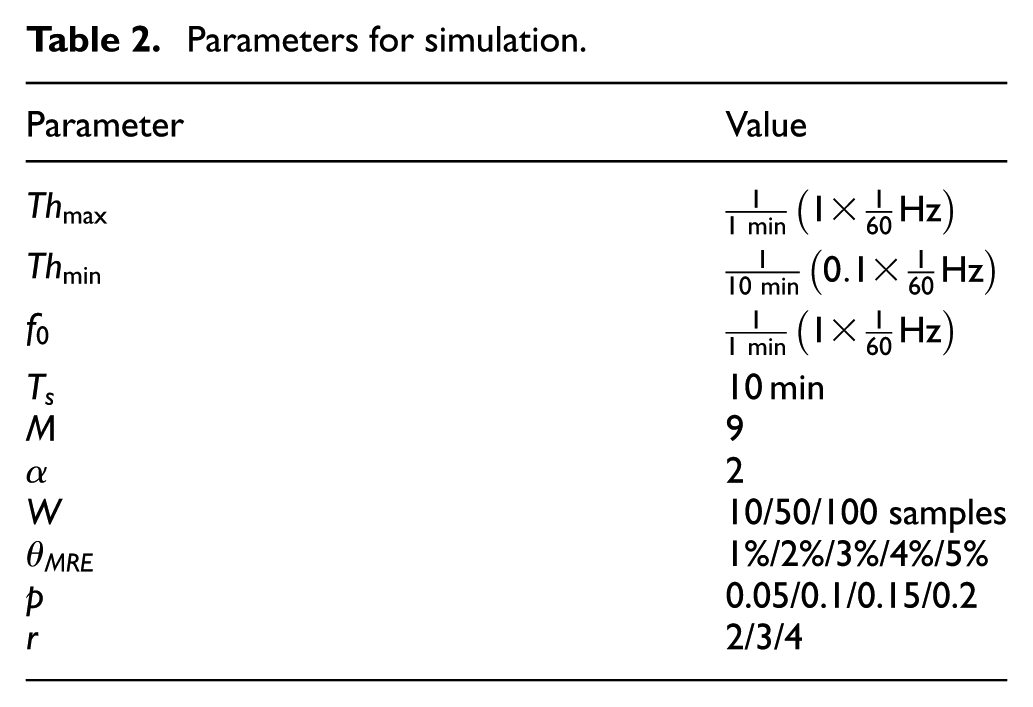
In this section, we describe the simulation settings and the metrics we have chosen to verify the performance of the proposed algorithm. MATLAB software³⁰ has been used for simulation tool. The evaluation metrics comprise correlation coefficient, predictive error, actual sampling frequency, and energy consumption rate. We compare performance with fixed sampling rate scheme, and the simulation process lasts 500 rounds to obtain average results. Table 2 demonstrates some important parameters for simulation.

Table 2.

Parameters for simulation.

Parameter	Value
$T h_{max}$	$\frac{1}{1 min} (1 \times \frac{1}{60} Hz)$
$T h_{min}$	$\frac{1}{10 min} (0.1 \times \frac{1}{60} Hz)$
$f_{0}$	$\frac{1}{1 min} (1 \times \frac{1}{60} Hz)$
$T_{s}$	$10 \min$
$M$	9
$α$	2
$W$	10/50/100 samples
$θ_{MRE}$	1%/2%/3%/4%/5%
$p$	0.05/0.1/0.15/0.2
$r$	2/3/4

It is assumed that each sensor node has the same initial energy 1 J, and energy consumption model is the same as Anastasi et al.,³¹ as such equations

E_{i}^{tx} = (e_{i}^{t} + ε_{amp} \times d^{2}) \times m; E_{i}^{rx} = e_{i}^{r} \times m

(13)

e_{i}^{t} = e_{i}^{r} = 50 nJ / bit; ε_{amp} = 100 pJ / (bit m^{2})

(14)

Simulation results and performance analysis

First, the criteria evaluation is introduced to measure spatial correlations between sensor nodes. The correlation coefficient equation is defined as follows

C_{uv} = | \frac{[D_{u} - \bar{E} (D_{u})] \times {[D_{v} - \bar{E} (D_{v})]}^{T}}{W \times \sqrt{Var (D_{u})} \times \sqrt{Var (D_{v})}} |

(15)

where $C_{uv}$ denotes correlation coefficient between $D_{u}$ and $D_{v}$ and $\bar{E} (D_{u})$ and $Var (D_{u})$ denote the average value and average square error of data sequence $D_{u}$ , respectively. $C_{uv} = - 1$ denotes that data sequences $D_{u}$ and $D_{v}$ are negatively related; $C_{uv} = 0$ denotes that data sequences $D_{u}$ and $D_{v}$ are irrelevant; and $C_{uv} = 1$ denotes that data sequences $D_{u}$ and $D_{v}$ are positively related. To calculate with 1 day data with the total length of 1100, the correlation coefficient of Sensor Nos 1 and 2 is 0.9393, while the correlation coefficient of Sensor Nos 1 and 16 is 0.7199. Therefore, the correlation coefficient value of Sensor Nos 1 and 2 is larger than that of Sensor Nos 1 and 16. However, in the specified spatial domain, the correlation values are different between Sensor Nos 1 and 2 (stronger correlation coefficient is 0.9393 when W = 100) and Sensor Nos 1 and 16 (weaker correlation coefficient is 0.7199 at W = 100) at different window sizes. It is obvious from these results shown in Figure 16 that there are strong spatial and temporal correlations of neighboring sensory data.

Figure 16.

Comparison of correlation coefficient with different window sizes: (a) window size, W = 10; (b) window size, W = 50; and (c) window size, W = 100.

Figure 17 compares the predictive error of Sensor No. 1 from 28 February to 29 February using AR model. We find out that predictive error is bounded by a certain small value, except that there is a major predictive error at boundary of 2 days due to some errors of original data set.

Figure 17.

Predictive error from 28 February to 29 February of Sensor No. 1: (a) temperature variation and (b) predictive error.

As a representative of energy consumption rate in sensory sampling process, the mean sampling frequency value Mean_f is defined as the ratio between the sum of actual sampling frequency with the number of sampling sequence as well as the unit of 1/60 Hz. It is obvious that the variation of sampling frequency drops from the original sampling frequency $T h_{max}$ in Figure 18. In other words, the instantaneous sampling frequency derived from our algorithm is a little smaller than fixed sampling, which is one unit average frequency. Therefore, the energy efficiency of whole WSNs has been improved. Moreover, the average sampling frequency will decrease when the MRE value increases.

Figure 18.

Sampling frequency self-regulation with different MREs.

The energy residual ratio is defined as the ratio between residual energy and initial energy of all sensor nodes in our simulations. Figure 19 illustrates simulation results of energy consumption ratio with different SCS granularity values and CH percents. The proposed ASbST algorithm achieves energy efficiency of data sampling by collecting sensory data from only a subset of sampler. The sensory data of non-sampler will be predicted using AR model derived from recent sensory data. It is very obvious from Figure 19 that energy consumption will increase with much larger cluster number because there are much more awake sensor nodes. Moreover, energy consumption with smaller SCS granularity is much greater than that of larger SCS granularity with the same reason.

Figure 19.

Energy consumption with different SCS granularity and cluster head percent.

Conclusion

In this article, we introduced an adaptive sampling algorithm based on temporal and spatial correlations for clustered WSNs. The proposed ASbST algorithm could be used to decrease data sampling frequency while guaranteeing data sampling quality efficiently. First, a novel clustering mechanism based on data gradient was proposed. Second, CHs maintained AR predictive model of sensory data in the time domain within each cluster, as well as self-adjusts and changes sampling frequency based on predictive model. Third, cluster members transmitted sensory data to its CH with self-adopting sampling frequency. Extensive simulation results verified that ASbST algorithm can achieve better performance with spatiotemporal correlations of historical sensory data. Our future work will focus on multi-dimensional sampling algorithm, which considers different spatial–temporal resolutions as well.

Footnotes

Acknowledgements

The authors would like to thank the anonymous reviewers whose insightful comments helped improve the presentation of this paper significantly.

Handling Editor: Amiya Nayak

Declaration of conflicting interests

The author(s) declared no potential conflicts of interest with respect to the research, authorship, and/or publication of this article.

Funding

The author(s) disclosed receipt of the following financial support for the research, authorship, and/or publication of this article: This research was partially supported by Natural Science Foundation of Zhejiang Province (No. LY18F030006 and No. LY16F030004) and National Natural Science Foundation of China (No. 61871163 and No. 61801431).

ORCID iD

Wenyu Cai

References

Gao

. Survey on sensor network research. J Comput Res Dev 2008; 45(1): 1–15.

Mainetti

Patrono

Vilei

. Evolution of wireless sensor networks towards the Internet of Things: a survey. In: 19th international conference on software, telecommunications and computer networks (SoftCOM), Split, 15–17 September 2011, pp.1–6. New York: IEEE.

Halil

Kent

TKC

Mohammed

et al . A survey of network lifetime maximization techniques in wireless sensor networks. IEEE Commun Surv Tut 2017; 19(2): 828–854.

Zesong

Bin

Shaoshi

et al . A survey of multi-objective optimization in wireless sensor networks: metrics, algorithms, and open problems. IEEE Commun Surv Tut 2017; 19(1): 550–586.

Anastasi

Conti

Francesco

et al . Energy conservation in wireless sensor networks: a survey. Ad Hoc Netw 2009; 7(3): 537–568.

Willett

Martin

Nowak

. Backcasting: a new approach to energy conservation in sensor networks. In: Information processing in sensor networks, Berkeley, CA, 26–27 April 2004, pp.124–133. IEEE.

Ordonez

Krishnamachari

. Optimal information extraction in energy-limited wireless sensor networks. IEEE J Sel Area Comm 2004; 22(6): 1121–1129.

Masoum

Meratnia

Havinga

PJM

. An energy-efficient adaptive sampling scheme for wireless sensor networks. In: The 8th IEEE international conference on intelligent sensors, sensor networks and information processing, Melbourne, VIC, Australia, 2–5 April 2013, pp.231–236. New York: IEEE.

Vuran

Akan

Akyildiz

. Spatio-temporal correlation: theory and applications for wireless sensor networks. Comput Netw 2004; 45(3): 245–259.

10.

Gedik

Liu

. ASAP: an adaptive sampling approach to data collection in sensor networks. IEEE T Parall Distr 2007; 18(12): 1766–1783.

11.

Aplippi

Anastasi

Francesco

et al . An adaptive sampling algorithm for effective energy management in wireless sensor networks with energy-hungry sensors. IEEE T Instrum Meas 2010; 59(2): 335–344.

12.

Santos

Dota

Cugnasca

. Dynamic definition of the sampling rate of data in wireless sensor network with adaptive automata. IEEE Lat Am T 2011; 9(6): 963–968.

13.

Zheng

Yang

Tian

et al . Data gathering with compressive sensing in wireless sensor networks: a random walk based approach. IEEE T Parall Distr 2015; 26(1): 35–44.

14.

Zhang

Cai

Zhou

et al . Energy-effective frequency-based adaptive sampling algorithm for clustered wireless sensor network. Lect Not El Engr 2014; 277(2): 107–114.

15.

Szczytowski

Khelil

Suri

. A Sample: adaptive spatial sampling in wireless sensor networks. In: International conference on sensor networks, ubiquitous, and trustworthy computing, Newport Beach, CA, 7–9 June 2010, pp.35–42. New York: IEEE.

16.

Deligiannakis

Kotidis

Roussopoulos

. Dissemination of compressed historical information in sensor networks. VLDB J 2007; 16(4): 439–461.

17.

. Data sampling control, compression and query in sensor networks. Int J Sens Netw 2007; 2(1): 53–61.

18.

Mukhopadhyay

Schurgers

Panigrahi

et al . Model-based techniques for data reliability in wireless sensor networks. IEEE T Mobile Comput 2009; 4(8): 528–542.

19.

Cheng

Cai

. O(ε)-approximation to physical world by sensor networks. In: The 32nd international conference on computer communications (INFOCOM), Turin, 14–19 April 2013, pp.3084–3092. New York: IEEE.

20.

Cheng

Hong

et al . Approximate physical world reconstruction algorithms in sensor networks. IEEE T Parall Distr 2014; 25(12): 3099–3110.

21.

Cai

Zhang

Jiang

. Coverage sampling technology based on spatial-temporal joint union for wireless sensor networks. Chin J Sens Actuator 2013; 26(2): 260–265.

22.

Jack

William

Jon

. Modeling and simulation for RF propagation. An introduction to network modeling and simulation for the practicing engineer. New Jersey: John Wiley & Sons, Inc. (IEEE Press eBook Chapters), 2011.

23.

Lotfinezhad

Liang

. Effect of partially correlated data on clustering in wireless sensor networks. In: International conference SECON, Santa Clara, CA, 4–7 October 2004, pp.172–181. New York: IEEE.

24.

Samuel

. Intel Berkeley Research Lab, http://bair.berkeley.edu/ (accessed January 2015).

25.

Zhang

Cai

Zhou

. A sensing data driven clustering algorithm for adaptive sampling in wireless sensor networks. Appl Mech Mater 2012; 182–183: 748–752.

26.

Sudharman

. Appendix A: Nyquist sampling theorem. In: Sudharman

(ed.) Signal processing for cognitive radios. Hoboken, NJ: Wiley (Telecom eBook Chapters), 2015, pp.704–710.

27.

Sun

Tao

. A constrained radial agglomerative clustering algorithm for efficient structure from motion. IEEE Signal Proc Let 2018; 25(7): 1089–1093.

28.

Najafi

Lahouti

Shiva

. AR modeling for temporal extension of correlated sensor network data. In: International conference on software in telecommunications and computer networks, Split, 29 September–1 October 2006, pp.117–120. New York: IEEE.

29.

Liu

Chen

Ding

. Generalized Yule-Walker blind identification for single-output multiple-output systems. In: The 32nd control conference, Xian, China, 26–28 July 2013, pp.1998–2001. New York: IEEE.

30.

MATLAB. The MathWorks Inc, http://www.mathworks.com/ (accessed October 2016).

31.

Anastasi

Conti

Francesco

et al . Energy conservation in wireless sensor networks. Ad Hoc Netw 2009; 7(3): 537–568.

Spatiotemporal correlation–based adaptive sampling algorithm for clustered wireless sensor networks

Abstract

Keywords

Introduction

Related works

Adaptive sampling for clustered WSNs

System model and overview

Adaptive sampling in the temporal domain

Adaptive sampling in the spatial domain

Clusters’ construction

ATS

ASS

ARMA-based predictive model at CH

Simulations and analysis

Simulation setup

Simulation results and performance analysis

Conclusion

Footnotes

Acknowledgements

Declaration of conflicting interests

Funding

ORCID iD

References