Sensor selection scheme in activity recognition based on hierarchical feature reduction

Abstract

To better understand the activity state of human, we might need multiple sensors on different parts of the body. According to different types of activities, the number and slot of required sensors would also be different. Therefore, how to determine the number and slot of necessary sensors regarding to wearers’ experience and processing efficiency is a meaningful study in actual practice. In this work, we propose a novel sensor selection scheme that is based on the improvement of the feature reduction process of the recognition. This scheme applies a hierarchical feature reduction method based on mutual information with max relevance and low-dimensional embedding strategy. It divides the process of feature reduction into two stages: first, redundant sensors are removed with one-order sequential forward selection based on mutual information; second, feature selection strategy that maximizing class-relevance is integrated with low-dimensional mapping so that the set of features will be further compressed. To verify the feasibility and superiority of the scheme, we design a complete solution for real practice of human activity recognition. According to the results of the experiments, we are able to recognize human activities accurately and efficiently with as few sensors as possible.

Introduction

For complex activities that involve movements of the whole body, one single wearable sensor is not enough in real applications. With the development of microelectromechanical system (MEMS), ¹ the cost of multiple-sensor systems has reduced considerably. Their application in human body activity estimation attracts much attention in related studies, since it is commonly believed that more sensors would bring higher accuracy. However, few researches consider the number and positions of essential sensors. As a matter of fact, this is a key problem that directly affects users’ experience. If we choose too many sensors, the recognition results would not improve much, while users’ comfort would be reduced. Meanwhile, proper positions of sensors are another important factor that needs to be considered. To detect different kinds of movements, we may need different number of sensors on different parts of the body. To save human cost with artificial intelligence, we try to learn this information with the assistance of the machine.

In this article, we discuss human activity recognition based on multiple wearable sensors and explore the best way to select the minimal needed number of features from the essential sensors. The key problem studied in this article is feature selection and reduction of multi-dimensional time series. Specifically, we focus on the following two questions:

• How to adaptively determine the number and positions of sensors according to different types of activities?

• How to improve feature selection and reduction mode to achieve better classification performance with as few features as possible?

To answer the first question, we attached a sufficient amount of sensors on different parts of human body as candidates and selected the essential ones according to their performance in learning actual activities. With prior experiment, we need to identify essential sensors that have strong correlations with the recognition result. Essential sensors and their positions are the key to our sensor configuration scheme. We define the problem as searching the best feature set NF from essential sensors in certain activity scene, and the definition of the problem is described below. To facilitate the understanding of the structure of the research object, a sensor is also indicated as a node in this article.

• Definition 1. Feature set of essential nodes NF: Given m sensors worn on different parts of the human body $S=\{S_1,S_2,\dots ,S_m\}$ , and the set of features extracted from these nodes indicated as $F=\{F_1,F_2,\dots ,F_m\}=\{f_1,f_2,\dots ,f_n\}$ . The essential nodes consist of the minimal set of sensors that keeps the recognition accuracy on the original level: $\mathrm{NS}=\{N{S}_1,N{S}_2,N{S}_{\mathrm{sm}}\},(\mathrm{NS}\subset S)$ . If we use $\mathrm{NF}=\{n{f}_1,n{f}_2,\dots ,n{f}_{\mathrm{nn}}\}$ to represent the best feature set, the combination of sensors should satisfy the following qualifications ( $\mathrm{accuracy}(F)$ returns the accuracy of classification using feature set $F$ , and $\xi$ is an extremely small value):

• $\mathrm{sm}\le m$ ;

• $\mathrm{nn}<<n$ ;

• $|\mathrm{accuracy}(F)-\mathrm{accuracy}(\mathrm{NF})|\le \xi$ ;

• $\forall j\in [1,nn],accuracy(NF\backslash \{n{f}_i\})<accuracy(NF)$ .

Since there are a large number of features obtained from many sensors, there must be redundant ones that have little influence on classification result; we need to reduce its scale to improve the performance of classification.

Aiming at the problem of the minimization of the number of nodes, the number of features, and the error rate of classification in the recognition process, we adopt the idea of feature reduction to determine the configuration of sensors and propose a hierarchical feature reduction method. First, we reduce the number of nodes in the first stage by applying a first-order forward searching mode based on mutual information (MI) queue, so that we can screen out sensors with high class-relevance and low mutual redundancy. Second, to solve the second question mentioned above, we select the features of the chosen nodes based on mixed feature selection model and reduce the dimensionality of the selected ones for the final features.

The rest of this article is organized as follows. In the “Related work” section, we discuss the related work of feature reduction in classification. In the “Hierarchical feature reduction with max relevance and low-dimensional embedding strategy” section, we introduce our solution for the problem described above. In the “The application and related experiments” section, we discuss the performance of our solution in actual practice of human activity recognition. And finally, we offer conclusions in the “Conclusion” section.

Related work

There are two common ways of feature reduction: feature selection and feature extraction. The first method chooses features with strong power of classification for soft data compression. The second method transforms the features to lower dimensional space from high dimension while keeping the original relationship between samples and classes unchanged.

There are basically three types of feature selection strategies, including filters, wrappers, and their combination. The filtering model evaluates the quality of feature candidates and chooses the best set of them. It does not involve any learning algorithm, what makes it more efficient. The quality of feature candidates mainly shows in two aspects: class-relevance and redundancy. Class-relevance indicates the relativity between the feature candidates and classes, while redundancy reflects the relationship between features. Methods like Laplacian score, ² Fisher score, ³ and RelifF ⁴ are commonly used in practice. These methods sort feature candidates according to their degree of correlation and screen out the proper ones by setting a threshold.

As for the redundancy between features, MI^5,6 is a common estimation. MI is often used to measure the amount of information that two random variables have in common. As a matter of fact, MI can measure not only the correlations between features but also the relations between features and classes. minimum Redundancy Maximum Relevance (mRMR) ⁷ is a typical example of using MI to estimation class-relevance and feature redundancy. It proposes an optimal first-order incremental selection mode that selects feature subsets with maximum dependency on classification results. This dependency is able to reflect the maximum correlation between features and classes as well as the minimum redundancy among different features. The feature subset we got from this algorithm is a set of features with maximum class-relevance and minimum redundancy. Maximum mean Discrepancy (MmD) ⁸ is a method that estimates the correlation between multiple features and classes using Renyi’s α-entropy. It builds up a minimum spanning tree ⁹ based on information entropy of features to perform the clustering of features and elimination of the outliers. These methods are quite efficient for ordinary data. However, they should be improved before their application to data with special structure.

As the filtering model is independent from the subsequent learning process, it might cause deviation and not able to find the proper feature candidates. To solve this problem, wrapping model^10,11 introduces a learning algorithm to measure quality of feature candidates. It measures the quality of feature candidates iteratively based on the cross-validation results of the classifier and finds out the suitable feature subset. Searching for the feature subsets during the learning loop is an NP-hard problem. Strategies like Hill Climbing, branch and bound, Greedy method, and genetic algorithm (GA) are commonly used to solve the problem.^12,13 There are basically three ways to find the subsets of feature candidates: full search, heuristic search, and random search. As the full search costs too much time, it is rarely used. The other two methods, however, are used more often as they are more efficient; for example, Sequential Floating Forward Selection (SFFS),^14,15 Particle Swarm Optimization (PSO),^16,17 and others. Since both models have their own advantages and drawbacks, their hybrid would be a proper trade-off. For instance, pruning strategy can be used to remove the irrelevant features in each iteration of the classification, ¹⁸ or we can combine logistic regression with linear classifier using regularization method. ¹⁹

Although the methods of feature selection are able to find out the representative features, the degree of reduction is limited by the original features. When features with strong class-relevance are found, it is especially difficult to improve the performance of classification with the remaining weak features. However, with the methods of feature extraction, we can further extract the abstraction of the original features. Low-dimensional embedding is a kind of feature transformation that preserves the distribution and correlations of samples in different classes.

There are three ways to find the low-dimensional embedding: unsupervised, supervised, and semi-supervised dimensionality reduction. Unsupervised dimensionality reduction preserves the distribution information of the samples without using their class labels. Algorithms like principal components analysis (PCA), ²⁰ kernel principal component analysis (KPCA), ²¹ unsupervised maximum margin projection (UMMP), ²² and kernel unsupervised maximum margin projection (KUMMP) ²³ are such kind of methods that are commonly used in many studies. Moreover, for nonlinear data, manifold learning such as locality preserving projection (LPP), kernel locality preserving projections (KLPP),^24,25 Laplacian eigenmaps (LE), ²⁶ locally-linear embedding (LLE), ²⁷ isometric feature mapping (ISOMAP), ²⁸ and stochastic neighbor embedding (SNE) ²⁹ are quite popular in recent years. They aim at keeping the distance relationship between neighbors, which maintains the characteristic of the manifold while mapping to lower space. Supervised dimensionality reduction, on the other hand, uses label information of samples. For example, linear discriminant analysis (LDA) ³⁰ and kernel linear discriminant analysis (KLDA) ³¹ choose the mapping direction that makes samples from the same class to be located as close together as possible, whereas samples from different classes stay far away from each other. relevant component analysis (RCA), kernel relevant component analysis (KRCA),^32,33 average neighborhood margin maximizing (ANMM), and kernel average neighborhood margin maximizing (KANMM) ³⁴ are also such kind of methods. Semi-supervised methods like semi-supervised dimensionality reduction (SSDR) ³⁵ and constraint margin maximization (CMM) ³⁶ are mainly used on data with only a few labeled samples.

With data transformation, we can achieve higher classification results with fewer features abstracted from the original ones. However, for data with certain structures, we cannot simply apply it to the original data directly. For example, in our situation, the primary task is to remove the redundant nodes so as to improve the users’ experience. As for the feature from the chosen nodes, low-dimensional embedding may help to improve the classification performance.

Hierarchical feature reduction with max relevance and low-dimensional embedding strategy

In practice of human activity recognition based on multiple sensors, one tricky problem is how to screen out the valuable and significant information from the obtained data. In some cases, human experience is not accurate enough to decide the optimal sensor configuration and the minimum key feature set for classification. In our study, we try to acquire the minimum key feature set using a feature reduction strategy. Feature reduction is an important part of classification process, especially in our situation, where we are facing data from a number of sensors. The relationship between the original features and our goal of feature selection are demonstrated in Figure 1. In this example, we demonstrate the scenario of five sensors with two features each. By choosing $\{f_2,f_5,f_9,f_{10}\}$ from $S_1$ , $S_3$ , and $S_5$ , we are able to achieve a fair performance. Thus, the two sensors represented by $S_2$ and $S_4$ are redundant nodes that should be abandoned. In such case, we cannot use the traditional structureless methods of feature selection directly.

Figure 1.

The tree structure of features with multi-nodes.

As the number of features in multi-nodes scenario is quite large, it is unwise to use the wrapping model directly. We mix the filtering and wrapping models to find the trade-off between efficiency and accuracy, so that we can receive better results in acceptable time. In this article, we propose a hierarchical reduction algorithm to extract features from data with multi-nodes structure. In the first stage of the method, we determine sensor configuration according to actual activities by selecting the essential candidates with a sufficient amount of information from a large enough number of sensors. The main idea is to build a sensor selection scheme that retains the essential nodes, while pruning the redundant ones. This process runs at the level directly under the root of the tree in Figure 1. For example, we choose sensors $S_1$ , $S_3$ , and $S_5$ . Features of the other two sensors are dropped. After getting a proper amount of sensors at the right place, we can identify the performed activities by classifying the data from these sensors. In the second stage of our method, before applying the classifier, we need to reduce the dimension of features using the max-relevance linear discriminant analysis (MRLDA) algorithm . This algorithm synthesizes the idea of feature selection and dimensionality reduction. This two-stage hierarchical solution is independent from the final classification and provides the freedom of choosing different classifiers according to the actual demands. In our example, $f_1$ and $f_6$ are abandoned, and the rest of the features are reduced to a lower dimension.

The first stage: nodes selection based on MI

In this part, we describe our sensor selection scheme that drops redundant sensors based on the idea of feature reduction. Specifically, we first line up the nodes in a queue based on their class-relevance, and put the head of the queue to the set of chosen candidates. Then, we successively select the nodes from the queue according to their relevance with the chosen ones in first-order incremental way. In this process, we need to check the classification performance every time an additional node is added and make sure its inclusion brings large enough benefit to the classification result.

In our solution, we use information entropy to indicate the correlation between feature candidates. Information entropy measures the uncertainty of a random variable, which shows the probability of a certain event. For random variable x, its entropy can be calculated as below

$$H\left(x\right)=-{\displaystyle \int p}\left(x\right){\log }_2\left(p\left(x\right)\right)dx$$

(1)

For any two random variables x and y, their joint entropy is shown below

$$H\left(\{x,y\}\right)=-\int \int p(x,y)·{\log }_{2}p(x,y)\mathrm{dx}\mathrm{dy}$$

(2)

This joint entropy has the following property

$$\max (H\left(x\right),H\left(y\right))\le H\left(\{x,y\}\right)\le H\left(x\right)+H\left(y\right)$$

(3)

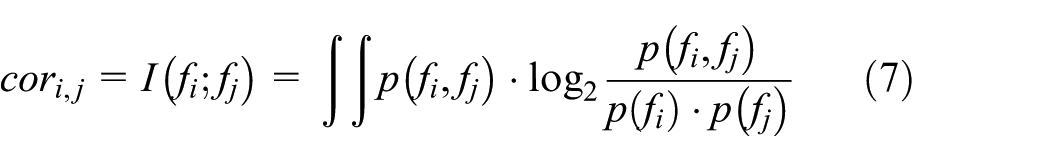
It represents the amount of the total information that contains in the combination of x and y. As for the relationship between two variables, MI is commonly used to do the measurement as follows

$$I\left(x;y\right)={\displaystyle \int {\displaystyle \int p}}\left(x,y\right)·{\log }_2\left(\frac{p\left(x,y\right)}{p\left(x\right)·p\left(y\right)}\right)dxdy$$

(4)

The MI between x and y can be understood as the amount of information that y and x have in common.

To improve selection efficiency of the wrapping model based on the first-order forward search, we estimate the class-relevance and the redundancy of each node during the search process. Results of the estimation are used to guide the search and to avoid unsupervised global search.

At the preliminary screening, we found out that it is practical to measure the class-distinguishing ability of each node with the MI between features of nodes and classes. Nodes with the higher mean value of the MI between features and classes possess stronger class-distinguishing ability, which we should choose preferentially during the selection process. Therefore, we build a queue with a length of m and put the nodes in the queue according to the order of their class-distinguishing ability.

While we give attention to the class-distinguishing ability of each node, we should not neglect their redundancy. If the existence of one node is unnecessary, it is in all probability that its features strongly related to features of other nodes. Therefore, we need to evaluate the correlation between the head of the queue and the chosen nodes during the selection process. We believe that the candidates with strong correlation with the chosen ones (the correlation with the chosen nodes larger than a certain threshold ${\eta }_c$ ) should be abandoned, so we label it and put it to the end of the queue. We iteratively select the candidates with weak correlation for cross-validation and choose the ones that improve classification accuracy while abandon the rest. If the accuracy achieves $\mathrm{accuracy}(F)$ or falls into an acceptable range, then we stop searching. For the labeled candidates, we do not need to check their redundancies when they get to the head of the queue again as they have already been checked before. In the worst case, all nodes are selected, which means that they all have their unique effect on the result and should be preserved.

In our study, we use the MI between the classes and all features of a certain node to estimate the class-distinguishing ability of the node. For one single feature $f_i$ and class $C$ , their MI is defined below

$$I(f_i;C)=\int \int p(f_i,C)·{\log }_2\frac{p(f_i,C)}{p\left(f_i\right)·p\left(C\right)}$$

(5)

Based on the assumption in related works, we obtain the class-distinguishing ability of node $S_j$ as

$$\mathrm{dt}{h}_j=\frac{\sum _{i=\mathrm{bn}\left(j\right)}^{\mathrm{en}\left(j\right)}I(f_i;C)}{\mathrm{en}\left(j\right)-\mathrm{bn}\left(j\right)+1}$$

(6)

Here, $\mathrm{en}(j)$ represents the first feature candidate of the jth node, and $\mathrm{bn}(j)$ represents the last feature candidate of the jth node.

As for the redundancy between different nodes, we can also perform the evaluation with the help of MI. For example, the correlation between two single features $f_i$ and $f_j$ can be defined as below

$$\mathrm{co}{r}_{i,j}=I(f_i;f_j)=\int \int p(f_i,f_j)·{\log }_2\frac{p(f_i,f_j)}{p\left(f_i\right)·p\left(f_j\right)}$$

(7)

Regarding the correlation between feature subsets of the nodes, we extended some related works. ⁷ For the set of feature candidates $F$ , we define the subset of feature candidates of node $S_1$ as $F_1=\{f_{\mathrm{bn}(1)},f_{\mathrm{bn}(1)+1},\dots ,f_{\mathrm{en}(1)}\}$ , the subset of feature candidates of node $S_2$ as $F_2=\{f_{\mathrm{bn}(2)},f_{\mathrm{bn}(2)+1},\dots ,f_{\mathrm{en}(2)}\}$ , and so forth. Then, we can define the feature correlation between nodes $S_x$ and $S_y$ as

$$\mathrm{co}{r}_{x,y}=\frac{\sum _{i=\mathrm{bn}\left(x\right)}^{\mathrm{en}\left(x\right)}\sum _{j=\mathrm{bn}\left(y\right)}^{\mathrm{en}\left(y\right)}I(f_i;f_j)}{\mathrm{en}\left(x\right)-\mathrm{bn}\left(x\right)+\mathrm{en}\left(y\right)-\mathrm{bn}\left(y\right)+2}$$

(8)

In this level, we select the nodes using the wrapping model with the first-order forward search method. Starting from the node with maximal class-distinguishing ability, we add one node with the highest class-relevance and lowest relevance with the chosen ones each time, and decide whether we should keep it according to the result of cross-validation until the ending criterion is satisfied. The pseudocode is shown below.

Algorithm 1.

$\mathrm{SelectNode}(F,C,m)$ .

Input: $F=\{F_1,F_2,\dots F_m\}$ is the set of feature candidates from all nodes, $m$ is the number of nodes.

Output: $\mathrm{CF}$ is the set of features from the chosen nodes.

1.  $\mathrm{CF}\leftarrow \varnothing$ ; $\mathrm{disAby}\leftarrow \varnothing$ ;

2.  $\mathrm{cand}\_\mathrm{node}\leftarrow$ initQueue $(-1,-1,0)$ ;

3. for $i\leftarrow i$ to $m$ do

4.   $\mathrm{dth}\leftarrow$ distinguishAbility $(F_i,C)$ ;

5.   $\mathrm{disAby}.$ add $(\mathrm{dth})$ ;

6. end for

7.  $\mathrm{idx}\leftarrow$ sortByQuality $(\mathrm{disAby})$ ;

8. for $i\leftarrow 1$ to $m$ do

9.  inQueue $(\mathrm{cand}\_\mathrm{note},\mathrm{idx}[i],0)$ ;

10. end for

11.  $\mathrm{pre}\_\mathrm{ary}\leftarrow$ crossValid $(F_{\mathrm{idx}[1]})$ ;

12. while !queueEmpty( $\mathrm{cand}\_\mathrm{node}$ ) do

13.   $\mathrm{cur}\_F\leftarrow$ deQueue $(\mathrm{cand}\_\mathrm{node})$ ;

14.  if $\mathrm{cur}\_f.\mathrm{sg}==0\&\&$ cor $(F_{\mathrm{cur}\_f},\mathrm{CR})>{\eta }_C$ then

15.   inQueue $(\mathrm{cand}\_\mathrm{node},\mathrm{cur}\_f,1)$ ;

16.  else

17.   $\mathrm{cur}\_\mathrm{ary}\leftarrow$ crossValid $(F_{\mathrm{cur}\_f}\cup \mathrm{CF})$ ;

18.  if $\mathrm{cur}\_\mathrm{ary}>\mathrm{pre}\_\mathrm{ary}$ then

19.   $\mathrm{CF}\leftarrow \mathrm{CF}\cup F_{\mathrm{cur}\_f}$ then;

20.  if $\mathrm{cur}\_\mathrm{ary}\ge \mathrm{ary}\_\mathrm{all}$ then

21.    break;

22.    else

23.  $\mathrm{pre}\_\mathrm{ary}\leftarrow \mathrm{cur}\_\mathrm{ary}$ ;

24.    end if

25.  end if

26.  end if

27. end while

28. Return $\mathrm{CF}$

After this selection, the redundant nodes are removed. However, there are still redundant feature candidates with weak class-distinguishing ability that exist in $\mathrm{CF}$ , and further feature reduction is carried out in the second stage.

The second stage: feature reduction based on MRLDA

As the ratio of feature compression is limited in the first stage, we can extract lower dimensional features without losing the information of the original ones by using the method of low-dimensional embedding in the second stage. But before this dimensionality reduction, we still need to drop some chosen features that do not contribute to the classification process. Therefore, in this stage, we propose a feature reduction algorithm called MRLDA. This algorithm brings dimensionality reduction into the process of feature selection by reducing the number of features, while maintaining the classification accuracy as well as improving classification efficiency. The operation of MRLDA is described below.

First, we estimate the class-relevance of each feature candidate with a filtering model of feature selection based on the MI between features and classes as well as among different classes. The selection of candidates with high class-relevance and low mutual redundancy, using first-order increasing selection mode, can approximately obtain a feature set with maximal class-relevance.

Second, following the rule that samples in the same class should be close to each other, while samples from different classes should be far apart, we get the transformation matrix of the feature set obtained in the first step for low-dimensional embedding.

Before we build the classifier for recognition, all data should be projected to lower dimension with the transformation matrix using MRLDA. The two important phases of this algorithm are described in detail in the rest of the section.

Selection of features based on class-relevance

According to the related definition and properties of information entropy, we can transform the goal of feature selection into the following optimization problem

$$maxI(\mathrm{CF};C)=maxI(\{c{f}_1,c{f}_2,\dots c{f}_{\mathrm{cn}}\};C)$$

(9)

As it is quite hard to solve this problem directly, some related studies use feature candidates with high class-relevance and low correlation between each other to approximate the features required. Thus, we select the features in each individual samples based on the estimation of their class-relevance and redundancy. Specifically, according to the property of MI, we have the following relationship

$$I(\mathrm{CF};C)=H\left(C\right)+H\left(\mathrm{CF}\right)-H(\mathrm{CF},C)$$

(10)

Mutual information between multiple features is represented in equation (11)

$$\begin{array}{c}\multicolumn{1}{c}{I_m\left(\mathrm{CF}\right)=\int \dots \int p(c{f}_1,\dots ,c{f}_{\mathrm{cn}}){\log }_2\frac{p(c{f}_1,\dots ,c{f}_{\mathrm{cn}})}{p\left(c{f}_1\right),\dots ,p\left(c{f}_{\mathrm{cn}}\right)}}\\ \multicolumn{1}{c}{\mathrm{dc}{f}_1,\dots ,\mathrm{dc}{f}_{\mathrm{cn}}}\end{array}$$

(11)

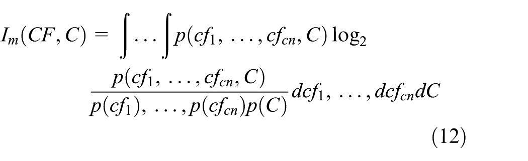
Similarly, we have MI between multiple features and classes as equation (12)

$$\begin{array}{c}\multicolumn{1}{c}{I_m(\mathrm{CF},C)=\int \dots \int p(c{f}_1,\dots ,c{f}_{\mathrm{cn}},C){\log }_2}\\ \multicolumn{1}{c}{\frac{p(c{f}_1,\dots ,c{f}_{\mathrm{cn}},C)}{p\left(c{f}_1\right),\dots ,p\left(c{f}_{\mathrm{cn}}\right)p\left(C\right)}\mathrm{dc}{f}_1,\dots ,\mathrm{dc}{f}_{\mathrm{cn}}\mathrm{dC}}\end{array}$$

(12)

Based on the relationship between MI and information entropy, we have the following equations

$$H\left(\mathrm{CF}\right)=\sum _{i=1}^{\mathrm{cn}}H\left(c{f}_i\right)-I_m\left(\mathrm{CF}\right)$$

(13)

$$H(\mathrm{CF},C)=H\left(C\right)+\sum _{i=1}^{\mathrm{cn}}H\left(c{f}_i\right)-I_m(\mathrm{CF},C)$$

(14)

If we insert equations (13) and (14) into equation (10), we get equation (15)

$$I(\mathrm{CF};C)=I_m(\mathrm{CF},C)-I_m\left(\mathrm{CF}\right)$$

(15)

To make computation easier, we use equations (16) and (17) to approximate $I_m(\mathrm{CF},C)$ and $I_m(\mathrm{CF})$ ⁷

$$I_m(\mathrm{CF},C)=\frac{1}{\mathrm{cn}}\sum _{i=1}^{\mathrm{cn}}I(c{f}_i;C)$$

(16)

$$I_m\left(\mathrm{CF}\right)=\frac{1}{2\mathrm{cn}}\sum _{i=1}^{\mathrm{cn}}\sum _{j=1}^{\mathrm{cn}}I(c{f}_i,c{f}_j)$$

(17)

It is proved by H Peng et al. ⁷ that feature subset selection can be optimized through first-order incrementally selecting features with maximal class-relevance and minimal redundancy among feature candidates. Therefore, we need to ensure that each time we choose a feature, it satisfies the term in equation (18). Assume that we have chosen $k$ features and saved in $S{F}_k$ , the next optimal feature candidate $\mathrm{sf}(k+1)$ would be added to $\mathrm{SF}$ and forms $\mathrm{SF}(k+1)$

$$s{f}_{k+1}=\underset{c{f}_i\in (\mathrm{CF}-S{F}_k)}{\mathrm{argmax}}[I(c{f}_i;C)-\frac{1}{k}\sum _{c{f}_j\in S{F}_k}I(c{f}_i;c{f}_j)]$$

(18)

In this way, features will be selected in the order of their classification accuracies and ultimately achieve convergence around the optimal result. With the sequential forward search (SFS) search mode, we find the best cutting position based on the feedback of the classifier. For instance, if the accuracy keeps rising, we will continue searching by successively adding new features into $\mathrm{SF}$ with sequential forward selection; otherwise, we will stop searching. And the features in front of current searching position will be the final choice recorded in $\mathrm{SF}$ .

After observing the changing of classification accuracy with different number of features, we discover that the accuracy rises rapidly with only a few features. However, as the number of features increases further, the upward tendency of the accuracy levels off with small variations. Although a few candidates with weak class-relevance often bring oscillation to the performance, more such candidates might bring another deterministic improvement. The algorithm with sequential forward selection mode might stop before it reaches the oscillation and cannot achieve better classification performance. But if we continue to add more new feature candidates, it would affect the efficiency. That means it is hard to ensure high accuracy and feature compression rate with current method alone. Hence, in our study, we keep the unstable candidates for second reduction phase.

Second reduction phase based on LDA

After selecting feature candidates from each node in the first phase, the reduction is still limited with limited compression of the chosen features. Therefore, in the second feature reduction phase, we project the chosen features from the first phase to lower dimensional space. To prepare features for classification, we need to find the best low-dimensional projection direction and then obtain the low-dimensional embedding of the testing data following this direction for classification during the recognition process.

To achieve this goal, we need to choose a method that supports exact extension outside of the training samples. Spectrum dimensionality reduction methods such as ISOMAP, LLE, and LE need Nyström approximation to find the rough projection direction. This projection often relies heavily on the actual training data as well as the local relations but may not suit the testing data. Besides, the label information of the training data is quite useful during the feature selection process in supervised learning.

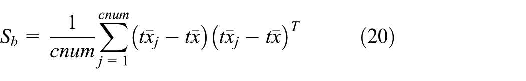
In the view of the analysis above, we choose the method of LDA for the second reduction phase. LDA is a typical supervised low-dimensional embedding algorithm. It searches the projection direction that maximizes inter-class distances and minimizes intra-class distances to reduce the dimension. Specifically, for the set of samples $\mathrm{TX}=t{x}_1,t{x}_2,\dots ,t{x}_{\mathrm{tn}}$ that belong to $\mathrm{cnum}$ classes, the intra-class dispersity is defined as

$$S_w=\frac{1}{\mathrm{cnum}}\sum _{\mathrm{cnum}}\frac{1}{n{m}_j}\sum _{X_i\in c_j}(t{x}_i-(t{\overline{x}}_j)){(t{x}_i-t{\overline{x}}_j)}^T$$

(19)

where ${\overline{x}}_j$ is the mean value of samples from the jth class. The inter-class dispersity is defined as

$$S_b=\frac{1}{\mathrm{cnum}}\sum _{j=1}^{\mathrm{cnum}}(t{\overline{x}}_j-t\overline{x}){(t{\overline{x}}_j-t\overline{x})}^T$$

(20)

where $\overline{x}$ is the mean value of all samples. Optimizing equation (21) with Lagrangian multiplier, we can get the transformation matrix $W_{\mathrm{opt}}$ that leads the best projection direction

$$W_{\mathrm{opt}}=\mathrm{argmax}\frac{|W^T{S}_{b}W|}{|W^T{S}_{w}W|}$$

(21)

In equation (21), the numerator is the inter-class dispersity after the projection, and the denominator is the intra-class dispersity after the projection. Through maximizing this objective function, we are able to find the projection direction that makes samples from different classes to be far away from each other while samples from the same class to be close to one another. This method is a sort of global dimensionality reduction. As we are able to obtain the transformation matrix and because the computation involves eigenvalue decomposition, it is easy to extend it to other data outside of current samples. Before the feature selection process, we set the number of features that are needed as $\mathrm{sm}$ and use NF to represent the final feature set that transformed from SF. The pseudocode of the second stage is demonstrated below.

Algorithm 2.

MRLDA ( $\mathrm{CF},C,k,\mathrm{nn}$ ).

Input: $\mathrm{CF}=c{f}_1,c{f}_2,\dots ,c{f}_{\mathrm{cn}}$ as the set of feature candidates from the chosen nodes, $C$ as the label information of samples, $k$ as the number of neighbors of features that determines the cutting position, $\mathrm{nn}$ as the number of final features.

Output: $W_{\mathrm{opt}}$ as the transformation matrix.

1.  $\mathrm{NF}\leftarrow \varnothing ;\mathrm{SF}\leftarrow \varnothing$ ;

2.  $\mathrm{mr}\leftarrow$ mrmr $(\mathrm{CF},C,\mathrm{cn})$ ;

3.  $\mathrm{SF}\leftarrow c{f}_{\mathrm{mr}(1)}$ ;

4.  $\delta \leftarrow$ threshold $(\mathrm{CF},k)$ ;

5.  $t\leftarrow 2$ ;

6. while $t<\mathrm{cn}$ do

7.   $\mathrm{cur}\_\mathrm{ary}\leftarrow$ crossValid $(\mathrm{SF}\cup c{f}_{\mathrm{mr}[t]})$ ;

8.  if $\mathrm{cur}\_\mathrm{ary}<\delta$ then

9.    $\mathrm{SF}\leftarrow \mathrm{SF}\cup c{f}_t$ ;

10.    $t\leftarrow t+1$ ;

11. else

12.  $\mathrm{SF}\leftarrow \mathrm{SF}\cup c{f}_t$ ;

13.  Break;

14.  end if

15. end while

16.  $W_{\mathrm{opt}}\leftarrow$ LDA $(\mathrm{SF},\mathrm{nn})$ ;

17. Return $W_{\mathrm{opt}}$

After obtaining the transformation matrix, we project the training and testing data to lower dimension where the classification takes place. Let $m_{\mathrm{SF}}$ and $m_{\mathrm{NF}}$ be the matrixes of $\mathrm{SF}$ and $\mathrm{NF}$ , we can get the final feature set $\mathrm{NF}$ using the equation below

$$m_{\mathrm{NF}}=W_{\mathrm{opt}}^T{m}_{\mathrm{SF}}$$

(22)

Construction of the classifier

There are many commonly used classifiers, such as k-NearestNeighbor (KNN), Bayesian model, ³⁷ support vector machine (SVM), ³⁸ Decision tree, ³⁹ and so on. KNN directly computes the distances between testing data and training data without building a model beforehand. It simply labels the testing data according to their nearest neighbors. Bayesian model calculates the posterior probability of an object with its prior probability using Bayesian statistical methods and finds the category it belongs to. Naive Bayes and Bayesian network are two common classifiers of this model. SVM finds a hyperplane that linearly separates samples from different classes with maximal margin and classifies them according to their positions projected on the plane. Through the transition of kernel function, we are able to get the embedding of samples in any high dimensions so that they can be linearly separated.

Apart from the single classifiers, ensemble learning is a paradigm that synthesizes the results of different classifiers. It also attracts much attention in related fields. At present, AdaBoost and Bagging ⁴⁰ are two such models that are frequently used. It is widely believed that the performance of AdaBoost is better than Bagging, while Bagging is more superior for data with noise. For the Bagging model, the greater diversities between the weak classifiers, the better performance we get from the ensemble classification. If the correlation between classifiers gets too strong, this model would face degeneration.

To improve the diversity of Bagging, the method called Random Forest ⁴¹ appears. This model builds a tree by random sampling with replacement in the training process. And it trains on each node by randomly selecting the subsets of the features in order to intensify the diversities between the nodes. In this way, we can efficiently prevent the over-fitting problem of the Decision tree model.

Rotation Forest ⁴² is another kind of ensemble learning based on Random Forest. It also focuses on building independent Decision tree on each node. But in this model, all samples of each node in the rotating feature space are used in training process. Each tree builds on the hyperplane that is parallel to the feature coordinate system. A totally different tree will be constructed if there is only a tiny little change in the rotation angle of the coordinate system. According to the studies of Rodriguez et al., ⁴² the performance of Rotation Forest is better than AdaBoost, Bagging, and Random Forest.

Ensemble learning combines advantages of various models and achieves better performances in most cases. However, its low time efficiency is one important problem we have to face. In the actual application, we need to balance the classification accuracy and time efficiency.

The application and related experiments

To check the feasibility of our solution, we apply it to the human activity recognition. Specifically, in the process of physical training monitoring, we need to recognize and analyze the motion patterns and activity state of the human body with wearable sensors. According to the actual requirements of this scenario, we can learn the configuration of sensors using our sensor selection scheme in the first stage of our solution with prior experiment. After that, we are able to identify different types of motion with the selected sensors using MRLDA in the second stage of our solution. In our case, we study 19 common activities in physical training. After given a sufficient number of sensors, we attempt to select the essential sensors to recognize the activities automatically.

To get more information of the movement of human body, we choose SensorTag devices to record the motion data. In each SensorTag, there is a three-dimensional accelerometer ( $A=\{A_x,A_y,A_z\}$ ), a three-dimensional gyroscope ( $G=\{G_x,G_y,G_z\}$ ), and a three-dimensional magnetometer ( $M=\{M_x,M_y,M_z\}$ ). Thus, we get nine groups of time series from one SensorTag device. In our experiment, we use more five SensorTag devices to record the movements on different parts of the human body, including both arms, both legs, and the waist. Together we have a 45-dimensional time series, which is shown in Table 1. In our study, we divide these time series into small fragments, each of which represents the sensing data within 5 s time frame. We define the small fragment as a sample in classification. In each fragment, we select the mean value and standard deviation of the time series in time domain as the feature candidates. Together we have 90 feature candidates in each sample.

Table 1.

Original time series of the five sensor nodes.

S	Body slot a	Time series
$S_1$	Left arm	$\mathrm{lm}\_a_x,\mathrm{lm}\_a_y,\mathrm{lm}\_a_z;\mathrm{lm}\_g_x,\mathrm{lm}\_g_y,\mathrm{lm}\_g_z;\mathrm{lm}\_m_x,\mathrm{lm}\_m_y,\mathrm{lm}\_m_z$
$S_2$	Right arm	$\mathrm{rm}\_a_x,\mathrm{rm}\_a_y,\mathrm{rm}\_a_z;\mathrm{rm}\_g_x,\mathrm{rm}\_g_y,\mathrm{rm}\_g_z;\mathrm{rm}\_m_x,\mathrm{rm}\_m_y,\mathrm{rm}\_m_z$
$S_3$	Waist	$\mathrm{wt}\_a_x,\mathrm{wt}\_a_y,\mathrm{wt}\_a_z;\mathrm{wt}\_g_x,\mathrm{wt}\_g_y,\mathrm{wt}\_g_z;\mathrm{wt}\_m_x,\mathrm{wt}\_m_y,\mathrm{wt}\_m_z$
$S_4$	Left leg	$\lg \_a_x,\lg \_a_y,\lg \_a_z;\lg \_g_x,\lg \_g_y,\lg \_g_z;\lg \_m_x,\lg \_m_y,\lg \_m_z$
$S_5$	Right leg	$\mathrm{rg}\_a_x,\mathrm{rg}\_a_y,\mathrm{rg}\_a_z;\mathrm{rg}\_g_x,\mathrm{rg}\_g_y,\mathrm{rg}\_g_z;\mathrm{rg}\_m_x,\mathrm{rg}\_m_y,\mathrm{rg}\_m_z$

a

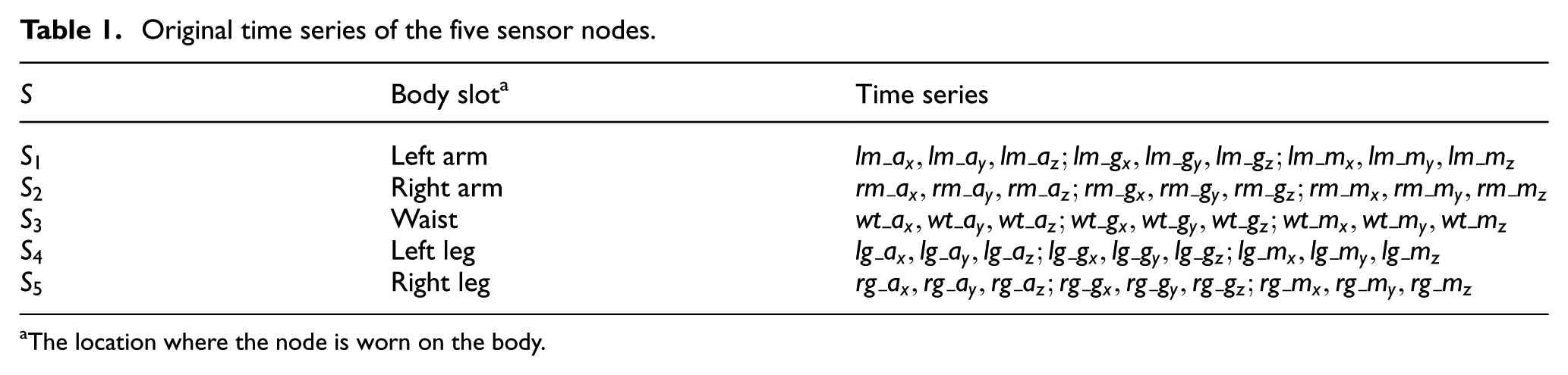
The location where the node is worn on the body.

Therefore, we build up a set of samples from 19 different classes. These classes represent the 19 types of common motion patterns of human body, including running, jogging, jumping, step training (going up and going down), deep squat, standing, sitting, walking, cycling, rowing, lying down, lying on the side, pitching practice, and five common warm-up exercises. These motions are chosen according to the actual need in real application. With the classification of the 19 classes, we are able to identify the specific ones from the 19 possible actions. In our experiment, each class contains 480 samples. We use fivefold cross-validation on the rest of the 7220 samples to test the classification performance. In this section, we are going to discuss this performance in three aspects:

• Performance of node reduction in the first stage

• Performance of feature reduction in the second stage

• Results of the recognition

Performance of node reduction

According to the result of our sensor selection scheme, we need only three sensors: $S_1$ , $S_2$ , and $S_5$ . That means we only need these three sensors on arms and legs to recognize and distinguish the 19 activities in our training, and only features from these three sensors can be used as candidates for the reduction in the second stage before classification. In this part, we compare the classification performance of the combination of our selected sensors to the other combinations that use more or less sensors.

Following the order of node selection, we check the classification accuracies with different number of nodes. Results are shown in Figure 2. The accuracy becomes acceptable when the number of features reaches 9 and yet still rising slightly using nodes labeled 1, 2, and 5.

Figure 2.

Classification accuracies with different amount of nodes: it is shown that the combination of sensors labeled 1, 2, and 5 is the best choice.

Regarding the number of selected nodes, we can see that if we use less than three nodes, the accuracy is clearly lower than other selection in most of the time. As for the situations of choosing more than three nodes, we do not receive better results than choosing only three nodes. Specifically, after the number of features reaches 9, choosing three nodes is superior to four or five nodes.

From these results, we can conclude that if the number of nodes is too small, the accuracy would be poor, whereas if the number of nodes is more than enough, we cannot see any advantages. For example, the accuracy of choosing all five nodes is not higher than accuracy of three nodes. So we can prove the effectiveness of our sensor selection scheme.

Performance of feature reduction

In this part, we check the feasibility and superiority of MRLDA by comparing its performance to other reduction methods. As we possess no apriori knowledge of the essential dimension of the features, we tried different projection of the feature set with maximal class-relevance in prior experiment to determine the dimension of the final features. In our solution, we get that 10-dimension is a stable state according to prior experiment. So the comparisons are done with 10 and less features.

First, to validate the effectiveness of the fusion in this stage, we compare the performance of MRLDA with mRMR ⁷ and LDA, ³⁰ and the results are shown in Figure 3. It is quite clear that the results of mRMR are inferior to the other two methods. That means that it is quite difficult to obtain good performance if we depend on pure selection from the original features, while the methods of low-dimensional embedding get better results. As we can see, the accuracy of MRLDA mostly grows faster and is better than that of the LDA.

Figure 3.

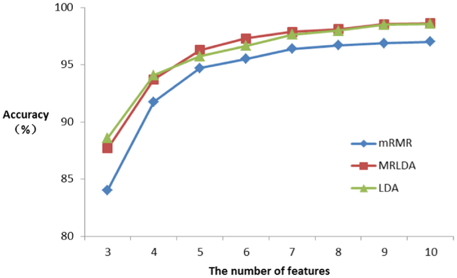
Classification accuracies with different methods of feature reduction in the second stage: the accuracy of MRLDA is the highest in most cases, followed by LDA and mRMR.

According to the results of the experiment, the accuracy is tending toward stability after the number of features reaches around 6. MRLDA reaches stability faster than the other two methods.

Second, to verify the superiority of the dimensionality reduction strategy of MRLDA, we choose the methods that can be extended outside of the data directly, such as PCA, ⁴³ LPP, ²⁵ and neighborhood components analysis (NCA) ⁴⁴ to reduce the dimensionality of the selected features from each node and compare their performance to MRLDA in Figure 4.

Figure 4.

Performances with different dimensionality reduction strategy: MRLDA has the highest classification accuracy, followed by MRLPP with a tiny gap, while the results of the other two methods are relatively much lower.

As the number of features increases, the growth rates of accuracy of all methods are declining. Among these methods, the result of MRLDA grows faster and keeps a highest record after the number of features reaches 5. Specifically, it is quite obvious that MRLDA is better than max-relevance neighborhood components analysis (MRNCA) and max-relevance principal component analysis (MRPCA). The results of max-relevance locality preserving projections (MRLPP) are quite close to MRLDA. In most cases (when the number of features is larger than 5), MRLDA performs the best performance. Meanwhile, MRLPP also performs quite well.

Except for the classification accuracy, time efficiency is also an important factor that we need to consider. Thus, we record the time consumption of MRLDA, MRPCA, and MRLPP in Figure 5. These results are obtained in the case of choosing 10 features.

Figure 5.

Time consumption of different methods.

Since NCA involves multiple iterations, the time consumption would be diverse with different amount of iterations. Moreover, its time consumption is much higher than the other three methods. For instance, it takes 138.92 s with at most 50 iterations to achieve the accuracy shown in Figure 4. Plus, its accuracy is lower than other methods in most cases. Thus, we do not discuss the performance of MRNCA in Figure 5.

Among these three methods, MRLPP takes the longest time. Although it is almost as accurate as MRLDA, it is not fast enough. MRPCA is the fastest but not accurate enough. Considering both classification accuracy and time efficiency, we believe that MRLDA is the best trade-off.

Results of the recognition

To estimate the performance of our solution in actual practice of human activity recognition, we try it on various classifiers such as Naïve Bayes, BayesNet, 1-NearestNeighbor (1-NN), Decision tree, SVM, Random Forest, and Rotation Forest. The results are described in Tables 2–5. The bold values in these tables are the best performance with different number of features.

First of all, we discuss the classification accuracies of its application in different classifiers, and the results are shown in Table 2.

Table 2.

Classification accuracies of different classifiers.

Number of features	Classifier
	BayesNet	Naïve Bayes	1NN	DT	RdF	SVM	RtF
3	76.87	70.46	86.63	85.17	85.96	88.48	88.14
5	90.48	81.73	96.67	93.45	95.98	96.55	96.51
7	94.58	89.74	97.95	94.88	97.41	97.84	98
10	95.66	92.01	98.6	95.58	98.14	97.88	98.78

DT: Decision tree; RdF: Random Forest; RtF: Rotation Forest; INN: 1-NearestNeighbor.

We can see from these results that the accuracies go up rapidly with the number of features, and this growth slows down after the number of features reaches 7. Among these classifiers, 1NN, SVM, and Rotation Forest behave quite well. Specifically, Rotation Forest gets the best performance with seven features.

Second, we check the precision with different amount of features in each classifier. The results are shown in Table 3.

Table 3.

Precision of different classifiers.

Number of features	Classifier
	BayesNet	Naïve Bayes	1NN	DT	RdF	SVM	RtF
3	76.1	71	86.2	84.7	85.6	88.2	97.7
5	90.5	82.5	96.6	93.4	96	96.6	96.4
7	94.6	90	98	94.9	97.4	98	97.9
10	95.7	92.3	98.6	95.6	98.1	98.2	98.8

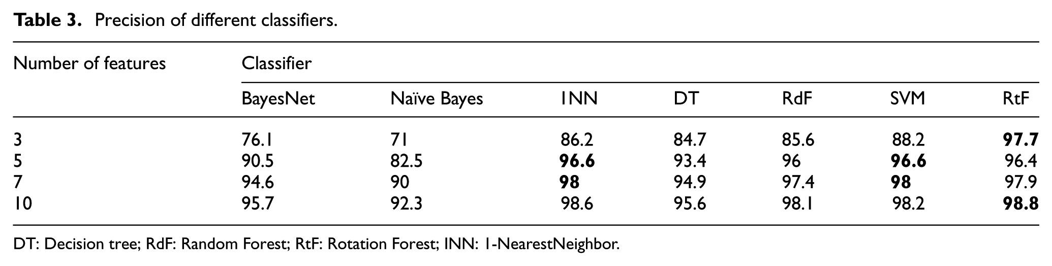
DT: Decision tree; RdF: Random Forest; RtF: Rotation Forest; INN: 1-NearestNeighbor.

According to the results, the superiority of Rotation Forest is quite obvious, as it is able to maintain high precision with different number of features. Other classifiers get higher precision with large number of features. The results become steady after the number of features reaches 7. SVM and 1NN also perform quite well.

Third, we discuss the recall rate with different number of features in Table 4.

Table 4.

Recall rate of different classifiers.

Number of features	Classifier
	BayesNet	Naïve Bayes	1NN	DT	RdF	SVM	RtF
3	76.9	70.5	86.6	85.2	86	88.5	88.1
5	90.5	81.7	96.7	93.4	96	96.6	96.4
7	94.6	89.7	98	94.9	97.4	97.8	97.9
10	95.7	92	98.6	95.6	98.1	97.9	98.8

DT: Decision tree; RdF: Random Forest; RtF: Rotation Forest; INN: 1-NearestNeighbor.

The performance of 1NN and Rotation Forest in recall rate is superior in general, and SVM is also quite good. The overall trend of all methods is still fast growth before 7 and becomes steady afterward.

Finally, let us take a look at the $F_b$ value ( $b=1$ ) in different situations. As we can see from Table 5, the superiority of Rotation Forest becomes more obvious after the number of features reaches 7.

Table 5.

$F_1$ of different classifiers.

Number of features	Classifier
	BayesNet	Naïve Bayes	1NN	DT	RdF	SVM	RtF
3	75.9	69.3	86.4	84.8	85.7	87.9	87.6
5	90.4	81.8	96.6	93.4	96	96.5	96.4
7	94.5	89.7	97.9	94.9	97.4	97.9	97.9
10	95.6	91.9	98.6	95.6	98.1	98	98.8

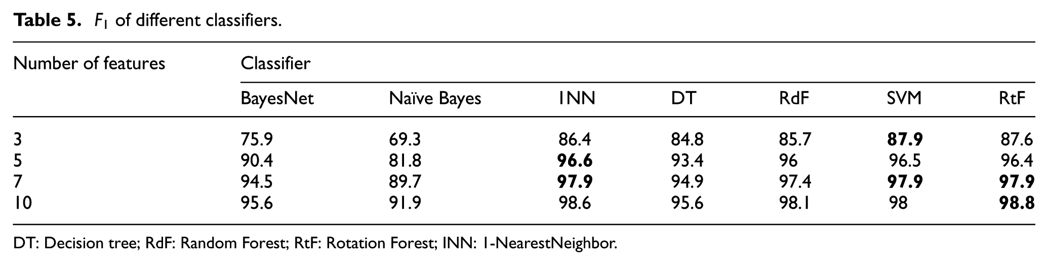
DT: Decision tree; RdF: Random Forest; RtF: Rotation Forest; INN: 1-NearestNeighbor.

To sum up, Rotation Forest did an excellent job in most cases, and the methods of ensemble learning are superior to single classifiers such as Decision tree and Bayes model. But in comparison to 1NN and SVM, their superiorities are not that obvious. After the comparison and balancing, we decided to select 10 features with our solution and use them with Rotation Forest classifier for use in the actual practice. In this way, we obtained a classification accuracy of 98.78% and compression rate of 88.89%.

Conclusion

In this article, we introduce a hierarchical feature reduction method that suits the classification of multi-dimensional movement sequences. By applying the idea of feature selection, we solved the problem of determining the required number and the body positions of multiple nodes. Through the related experiments, we proved the feasibility of our solution and found the balance between users’ experience and recognition accuracy. Meanwhile, combining the merits of feature selection and dimensionality reduction, MRLDA not only achieves accuracy that is better than with the other two methods but also improves the compression rate of feature selection as well as calculation efficiency. From the results of its application in human activity recognition, we are able to confirm its effectiveness and usability in real practice.