Sage Journals: Discover world-class research

Abstract

Due to energy limitation in wireless sensor networks, clustering is an efficient scheme which has been widely used in building practical wireless sensor networks, and various cluster head selection methods have been proposed nowadays. However, less emphasis was placed on the application constraints cluster head selection. In traditional clustering wireless sensor networks, cluster head is always located at the cluster centre and cannot detect an intruding target since the target first transits the border. Moreover, the data sensed from a target are sent by each cluster head through different routings to the sink so that it cannot be aggregated efficiently near the data source. In order to address these problems, this article proposes an efficient target tracking approach, in which the nodes on the edge of a cluster instead of the centred nodes are chosen as cluster heads so that cluster heads can serve as manager and monitoring node. Furthermore, we choose a collecting cluster head to collect the sensed data from the cluster heads around the target to facilitate data aggregation. Hence, the sensed data can be aggregated near to the data source, which avoids the data long-distance transmission and reduces data gathering costs. Moreover, each cluster head has different lifetime in the efficient target tracking approach according to its location and residual energy to balance the energy cost. Experimental results show that efficient target tracking approach outperformed the state-of-the-art approaches by improving the energy consumption as well as prolonging the network lifetime by about 20% as the 20% nodes die.

Keywords

Energy efficiency cluster head selection application constraints data collection monitoring and tracking

Introduction

Wireless sensor networks (WSNs) have been widely used as a desirable technology that can gather information by the cooperation of abundant sensor nodes. In WSNs, one of the important applications is target monitoring and tracking, such as vehicle tracking, damage detection^1,2 or structural health monitoring,^3,4 and monitoring migration behaviour of animals. Nowadays, this field has attracted the significant attention of many researchers.^5–7 Since sensor nodes are usually located in natural and unaccompanied environments, thus it is impossible to recharge their battery. Therefore, saving energy is crucial in the design of the network protocols.

Clustering is an efficient approach to save energy because only cluster heads (CHs) need in work status and the most of nodes can sleep. CHs are responsible for sending the sensed data to the base station and should always keep active. In addition, clustering is also a good way to solve the capacity and scalability problems to reduce data transmission collisions.^8,9 For example, low-energy adaptive clustering hierarchy (LEACH),¹⁰ is one of famous clustering protocols, in which CH is elected randomly and periodically. In the existing works, although CH is in active state, it cannot detect a target appeared on the edge of the cluster since CH always is located at the cluster centre. Nevertheless, in target tracking application, if a target moves into a cluster sensing range, it will first transit the cluster border. If CH wants to know whether a target is about to enter the cluster territory or not, one way is it receives the target information from other CHs or from the sink. As we know, communicating for sensor nodes has much more energy consumption than sensing; thus, CH relied on distant communication for target information usually consumes a lot of energy. The other way is the cluster border nodes have to keep active to get ready for detecting (as shown in Figure 1(a)) and provide the target information to help their CH to manage the sleep time of the cluster members. This way also causes unnecessary energy consumption. In addition, a target is usually sensed by the sensor nodes in multiple clusters and each CH sends the sensed data to the sink through different routings. Therefore, the data sensed from a target cannot be efficiently aggregated until it arrives at the sink and that could cause large amounts of redundant data to be transmitted in the network. Thus, considering application constraints is very useful to optimize target tracking WSNs. Application constraints in this article means that we used some characteristics of the target tracking application scenario to restrict the protocol of the CH selection and data collection so that the network performances are improved.

Figure 1.

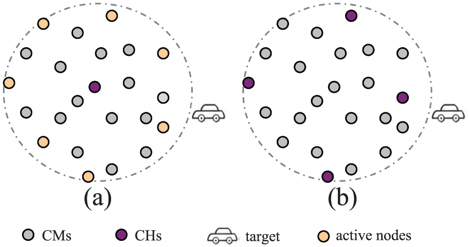
Illustration of target tracking in the different cluster schemes: (a) traditional cluster scheme and (b) ETTA cluster scheme.

With these motivations, this article proposes an efficient target tracking approach called ETTA, based on dynamic CH selection, in which we dynamically choose four nodes located on the edge of a cluster to play the roles of CHs. One cluster is further divided into four sub-areas by the four CHs. After that, each node is registered as the member of the nearest CH. Consequently, CHs could take the double roles both manager and detecting nodes so that the network could meet the requirement of the target tracking performances on condition that the fewer nodes keep active. Furthermore, to balance energy consumptions on each node, an adaptive CH re-selection scheme is proposed to allow each CH has different lifetimes according to the CH location and residual energy. Besides, a collecting cluster head (CCH) is chosen from the CHs near the target to collect the sensed data, and which facilitates the sensed data aggregation and avoids the long-distance transmission of large amounts of data. As a result, the proposed ETTA has high energy efficiency and could decrease energy costs of data transmitting to extend the lifetime of networks. In contrast to existing works, the contributions of this article include the following:

High energy efficiency: CH is dynamically chosen on the edge of a cluster to play the roles of both CH and detecting node so that CH has high energy efficiency.

Adaptive energy consumption balancing: each CH has different lifetimes in the light of its residual energy and communication costs. If CH lifetime expires, new CH will be chosen. Then the previous CH becomes cluster member.

Efficient data collecting: after each CH receives the sensed data from its members, it sends the data to CCH instead of relay nodes. Thus, the sensed data could be aggregated as soon as possible, and the workload of data transmission as well as the energy cost is reduced.

Related works

Recently, some clustering algorithms and data collecting protocols have been proposed. For clustering sensor network, a typical and energy-efficient hierarchical protocol is LEACH,¹⁰ which divided the whole network into multiple clusters and a node is selected as a CH. The nodes in one cluster take turns as the CH to avoid imbalanced energy consumptions. CHs are responsible for collecting the sensed data from their members and reporting the data to the sink.

The literature¹¹ proposed a novel network construction and routing method by defining three different duties for sensor nodes, that is, node gateways, CHs and cluster members. And then a hierarchical structure from the sink to the normal sensing nodes was applied. Although the method provides an efficient rationale to support the maximum coverage, the selected CHs may not be distributed evenly. The literature¹² proposed a hybrid approach for CH selection in which both residual power and communication consumptions are considered to choose the CH. The literature¹³ proposed an improved version of the energy aware distributed unequal clustering protocol (EADUC) to solve energy hole problem in multi-hop WSNs. EADUC elected CHs considering number of nodes in the neighbourhood to compute the competition radii and provide better balancing of energy. Moreover, the data transmission phase has been extended in every round by performing the data collection number of times through use of major slots and mini-slots. The literature¹⁴ proposed a randomness data regeneration approach for CH selection. The goal of this work is to select CH within a cluster based on the random locations of the sensor nodes. The authors took the power heterogeneity of the nodes into account and each cluster had several vice-heads, which can replace the CH later when the current CH uses up its energy.

In the above-mentioned literatures, CH was elected by many kinds of methods; also lots of influential factors for CH election were considered, such as the residual energy of nodes, the distance between nodes and the deployed density of nodes. Although these methods could provide energy efficiency in some cases, the application constraints were not considered in CH election. These methods are not suitable for the target tracking applications because the CHs always were located at the centre of a cluster. If the CH wants to know the information of the target appeared on the edge of the cluster, it has to communicate with other nodes so as to consume more energy. In addition, the CH keeps active and just manages its members, but not a detecting node; thus, it has low energy efficiency.

For data collecting in clustering WSNs, Node Density-based Clustering and Mobile Collection (NDCM) approach was proposed in Zhang et al.,¹⁵ which combines the hierarchical routing and mobile elements data collection. The authors proposed a CH selection scheme based on the node density so that a node at the centre of a densely nodes deployed area is to be a CH. The CHs first gather information from the cluster members and then the mobile element visits these CHs to collect data. Despite NDCM can improve the efficiency of both intra-cluster routing and data collection, it brought more latency because CHs had to wait for the mobile element. In Abid et al.,¹⁶ the authors proposed a hybrid method that combines multi-level clustering and structure-free algorithm for real-time WSN applications. Moreover, they adopted an event-driven CH election algorithm to rotate the CH role. Unfortunately, the multi-level clustering structure cannot adaptively change as the target moves.

In Chang et al.,¹⁷ the authors proposed a dynamic hierarchical protocol based on combinatorial optimization (DHCO) to balance energy consumption of sensor nodes and to improve WSN longevity. DHCO algorithm established a feasible routing set for each sensor node instead of selecting the CH or the next hop node to obtain the optimal route, which was formulated as a combinatorial optimization problem. In Estévez et al.,¹⁸ the authors proposed a routing algorithm based on a dynamically allocated hierarchical clustering, which used the link quality indicator as a reference parameter, maximizing the network coverage and minimizing the control message overhead and the convergence time. This work allowed for the application of complex management techniques and the algorithm had a fast setup time, a reduced overhead and a hierarchical organization.

Dynamic clustering algorithms and mobile elements data collection have some flexibility and adaptability in the existing works; nevertheless, these approaches cannot avoid the data sensed from a target to be sent through different routings, which leads to inefficient data aggregation and more energy consumption. By contrast to the existing approaches, ETTA proposed in this article concentrates on getting higher energy efficiency for choosing CH and collecting data by considering application constraints.

Efficient CH selection approach

Network model and evaluation indexes

In this article, the sensor network includes a sink and many sensor nodes (N_i, i ∈ [1, 2, 3,… ]) deployed in a two-dimensional sensing field A × B. Our sensor network model has the following properties and assumptions:

The sink is static and located far from the network. Moreover, it is responsible for the data collection from sensing fields and it has continuous power provision.

All sensor nodes are homogeneous and energy constrained. The distribution of sensor nodes is mutually independent. The nodes are stationary after deployment and equipped with a Global Positioning System (GPS) unit to know their positions. Let N_i(x_i, y_i) be the location of node N_i.

The network is organized into clusters. Each cluster has four sub-clusters and each sub-cluster has a CH and a number of cluster members (CMs). CH manages its CMs. CHs keep active all the time and they are replaced by CMs periodically.

When a target moves into the deployed area, the nodes detect the target periodically and send the sensed data to their CH.

CMs have sleep and active states. If there is no target in the sensing range of a cluster, the CMs are in the sleep mode most of the time and wake up for a fraction of the time to receive the task assignment messages from their CHs. If there is a target, the CMs keep active to track the target.

To balance the energy consumption, the sink will start the process of the cluster reforming after a specific period of time and then the nodes reform clusters in the same time. At other times, clusters are asynchronous and CHs election can be negotiated in a cluster.

Furthermore, sensor nodes have two modes, active or sleep, from which we could obtain the duty cycle γ of the node, which is the ratio of the time in active mode to a total data period. In detail, the active state includes work and idle states. In work state, nodes sense a target, send or receive data, while in idle state, nodes do not detect any target and just listening and receive message from others. In sleep mode, the sensor node could not execute any function, and it could not be woken up externally, instead had to set internal timers to determine the next time to come awake. In general, sensor nodes mainly consume energy in data receiving and transmitting, and idle listening when they are in active mode.

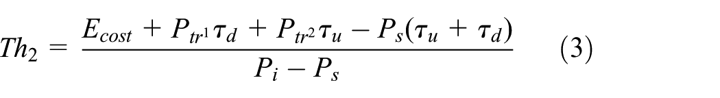
Figure 2 shows the power-time curves for transition of the node states. Active, idle and sleep states have power consumption P_a, P_i and P_s, respectively. The transition time to it from active state and back are denoted by τ_d and τ_u, respectively. From that we can see sleep state has less power consumption but incurs a latency and energy to awaken. Assume an event is detected by node N_i at some time. N_i finishes processing the event at time t₁ and predicts the next event occurs at time t₂ = t₁ + t_i. At time t₁, N_i decides if it transfers to sleep. Therefore, a sleep time threshold T_{th, k} can be utilized to avoid losing event

T h_{1} = τ_{d} + τ_{u}

(1)

Figure 2.

Sleep states transition latency and power.

If (t₂ – t₁) > Th₁, N_i can go to sleep state at time t₁ and wake up at t₂. Otherwise, when (t₂ – t₁) ≤ Th₁, N_i should not. Therefore, the saving energy from a state transition can be calculated as follows

E_{save} = P_{i} t_{i} - P_{t r^{1}} τ_{d} - P_{t r^{2}} τ_{u} - P_{s} (t_{i} - τ_{d} - τ_{u})

(2)

The energy saving makes sense when E_save > E_cost, where E_cost is the additional energy consumption for the sleep states transition, and $P_{t r^{1}}$ and $P_{t r^{2}}$ are the power consumption in the transition state from active to sleep state and back, respectively. Therefore, we can find out the threshold

T h_{2} = \frac{E_{cost} + P_{t r^{1}} τ_{d} + P_{t r^{2}} τ_{u} - P_{s} (τ_{u} + τ_{d})}{P_{i} - P_{s}}

(3)

In order to evaluate the performance of the network, the following definitions are defined in this study:

Average transmission delay (ATD): the first evaluation index defined in this article refers to the real-time performance of the target tracking network. ATD is the duration from the time when the nodes sensed a target to the time when the sink receives the enough sensed data which can be used to locate the target and aware its moving status. According to the three-point positioning principle, in order to determine the position of the target, the target is sensed by more than three nodes at the same time, that is, the target is in the k-coverage state (k ≥ 3). The smaller the ATD, the better the network tracking performance, that is, the network can quickly obtain the target location and moving status.

Tracking successful rate (TSR): the second evaluation index defined in this article refers to the tracking performance. We assume the successful tracking is that the target is sensed by more than three nodes at the same time. Therefore, TSR is defined as the ratio of t to T in the tracking procedure, that is, TSR = t/T, where t denotes the time duration the target is in the k-coverage state (k ≥ 3), and T illustrates the total time of the target in the monitoring area.

Average energy consumption (AEC): the third evaluation index defined in this article refers to the energy efficiency of the system. AEC is defined as the AEC of all the nodes in the tracking process, when the target moves through the monitoring region.

Network lifetime span (NLS): the last evaluation index defined in this article refers to the network lifetime. NLS is defined as the time when the first node dies or a certain percentage of nodes die in the network.

The main goal of the node scheduling and CHs selection algorithm are proposed in this article is trying to reduce AEC and prolong NLS on the premise of low TD and high TSR.

Network initialization and dynamic CHs selection

Initially, as shown in Figure 3(a), the sensing area is divided into m × n smaller areas, which are regarded as clusters. Each cluster is differenced by its cluster identification, Id(C_j) = (u_j, v_j). Each node N_i decides which cluster it is in by the coordinate N_i(x_i, y_i) like the following

u (N_{i}) = [\frac{x_{i} - x_{0}}{A / m}], v (N_{i}) = [\frac{y_{i} - y_{0}}{B / n}]

(4)

where [X] represents to only pick out integer part of the figure X. (x₀, y₀) is coordinates of origin. The nodes in one cluster have the same cluster identification.

Figure 3.

Illustration of forming cluster structured sensor network: (a) forming cluster structure and (b) reforming cluster structure.

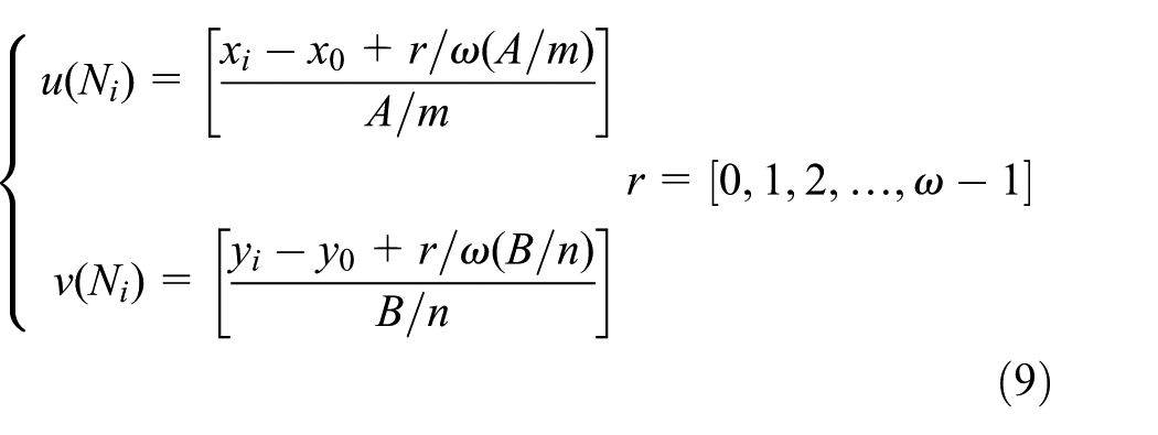
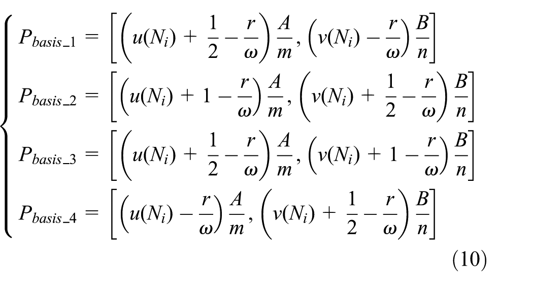
After dividing the network into cluster, the procedure of electing CH is started. We select four nodes in one cluster as the CHs which are located at the centre of the edges of each small area. In this way, each CH is not only a manager but also a detecting node. Thus, the energy efficiency is improved. The step of CH election is shown as follows.

First, each node calculates the coordinates of the basis CH points which are midpoints of four edges of a cluster. The calculations are

{\begin{matrix} P_{basis_1} = [(u (N_{i}) \frac{A}{m} + \frac{A}{2 m}), v (N_{i}) \frac{B}{n}] \\ P_{basis_2} = [(u (N_{i}) + 1) \frac{A}{m}, (v (N_{i}) \frac{B}{n} + \frac{B}{2 n})] \\ P_{basis_3} = [(u (N_{i}) \frac{A}{m} + \frac{A}{2 m}), (v (N_{i}) + 1) \frac{B}{n}] \\ P_{basis_4} = [u (N_{i}) \frac{A}{m}, (v (N_{i}) \frac{B}{n} + \frac{B}{2 n})] \end{matrix}

(5)

Second, one cluster is divided into four sub-clusters and each sub-cluster was defined in the area of the cluster edge. Then, each node calculates the distance to the each basis CH point in a cluster and registers itself to the nearest sub-cluster $C_{sub_p}, p \in [1, 2, 3, 4]$ .

Finally, each node in the sub-cluster competes for CH and one CH is chosen in each sub-cluster. The node, which is nearest to the basis CH point and has more residual energy in the sub-cluster, is selected as the CH. In a process of CH election, each node N_i broadcasts an announcement ‘elect_CH’ after waiting for a time period T(N_i)

T (N_{i}) = T_{\min} + (T_{\max} - T_{\min}) F (N_{i}) + T_{ran}

(6)

F (N_{i}) = λ \frac{d | N_{i}, P_{basis_p} |}{max {A / 2 m, B / 2 n}} + (1 - λ) \frac{E_{ini} (N_{i}) - E_{res} (N_{i})}{E_{ini} (N_{i})}

(7)

where T_min denotes minimum waiting time and T_max is maximum waiting time. These two parameters are utilized to avoid the waiting intervals too long or too short. T_ran is different for each node and it is a discrete random variable with the uniform distribution in [10⁻⁴, 10⁻⁵], and it is generated by an each node internal controller. T_ran is an order of magnitude smaller than T_min and added to prevent the collision caused by the same distances or residual energy of two nodes. $F (N_{i})$ is a function of the residual energy and distance of node N_i. In $F (N_{i})$ , $λ$ is the distance weight which indicates the distance influence to the waiting time, and $0 \leq λ \leq 1$ . $d | N_{i}, P_{basis_p} |$ is the distance between node N_i and $P_{basis_p}, N_{i} & & P_{basis_p} \in C_{sub_p}$ , $p \in [1, 2, 3, 4]$ and $E_{ini} (N_{i})$ are the residual and initial energy of N_i, respectively. When the waiting time $T (N_{i})$ expires, the node N_i broadcasts the announcement ‘elect_CH’ to others. If the node in the same sub-cluster receives the announcement message, it will cancel the waiting time and give up the election of CH to guarantee just a CH in one sub-cluster.

Cluster maintenance

To avoid excess energy consuming on CH, each CH has different lifetime according to its residual energy. The CH_j lifetime value is calculated as follows

L (C H_{j}) = δ_{\min} + δ_{e_ref} \frac{E_{res} (C H_{j})}{\bar{\sum_{n_{i} \in C_{sub_p}} E_{res} (n_{i})}}

(8)

where $L (C H_{j}) \in [0, 1, 2, \dots]$ , it indicates the number of the sensed data collecting rounds. $δ_{\min}$ is the minimum lifetime and $δ_{e_ref}$ is the energy-related reference value of CH lifetime. $E_{res} (C H_{j})$ is the residual energy of CH_j. $\bar{\sum E_{res} (n_{i})}, n_{i} \in C_{sub_p}$ is the average residual energy of the nodes which are in the same sub-cluster with CH_j. Thus, the more residual energy the node has, the longer it serves as CH. The lifetime information of the CH_j is included in the CH announcement message informed to all the cluster members who send the sensed data to their CH each time and update $L (C H_{j}) = L (C H_{j}) - 1$ , until $L (C H_{j}) = 0$ , and then, CH_j informs all the members to start a new round of CH election.

After a period of data collection, the nodes located at the edge of a cluster consumed more energy. To balance the energy consumption, the sink will start the process of the cluster reforming after a specific period of time. The area of one cluster will be assigned again as Figure 3(b) shows. Each node N_i determines which cluster it is in once again by the following equations

{\begin{matrix} u (N_{i}) = [\frac{x_{i} - x_{0} + r / r ω ω (A / m)}{A / m}] \\ v (N_{i}) = [\frac{y_{i} - y_{0} + r / r ω ω (B / n)}{B / n}] \end{matrix} r = [0, 1, 2, \dots, ω - 1]

(9)

where $r / r ω ω (A / m)$ and $r / r ω ω (B / n)$ denote the distance of a cluster boundary line moved along the x- and y-axis, respectively, that means a cluster side length ( $A / m$ or $B / n$ ) is divided into $ω$ equal parts, and in the current period, the number of the equal parts is $r$ . After the $ω$ time periods, the cluster boundaries move a cluster side length to the left or up. In this way, the nodes on the edge of a cluster in the previous time period will be converted to the interior nodes of the cluster in the current time period so that the energy consumption is balanced. Correspondingly, each node calculates the coordinates of the basis CH points as follows

{\begin{matrix} P_{basis_1} = [(u (N_{i}) + \frac{1}{2} - \frac{r}{ω}) \frac{A}{m}, (v (N_{i}) - \frac{r}{ω}) \frac{B}{n}] \\ P_{basis_2} = [(u (N_{i}) + 1 - \frac{r}{ω}) \frac{A}{m}, (v (N_{i}) + \frac{1}{2} - \frac{r}{ω}) \frac{B}{n}] \\ P_{basis_3} = [(u (N_{i}) + \frac{1}{2} - \frac{r}{ω}) \frac{A}{m}, (v (N_{i}) + 1 - \frac{r}{ω}) \frac{B}{n}] \\ P_{basis_4} = [(u (N_{i}) - \frac{r}{ω}) \frac{A}{m}, (v (N_{i}) + \frac{1}{2} - \frac{r}{ω}) \frac{B}{n}] \end{matrix}

(10)

In addition, the following CH selection and cluster maintenance steps are the same as those mentioned above, and we are no longer repeated here.

Sensed data transmission

If a target moves into the deployed sensing area, CHs will wake up the corresponding members to active state. Each active node sends its sensed data to its CH. Then the CH aggregates the data and transmits it towards the sink according to the specified routing algorithm. However, different CHs always transmit data to the sink through the different routings, the sensed data from a target cannot be aggregated before these data arrive the sink (as shown in Figure 4).

Figure 4.

Data transmitting in clustering networks.

In target tracking scenario, the sensed data from vicinity area have strong correlations due to the high density of sensors, and normally, many sensors record the information of a single target. If more CHs transmit the data sensed from a target through different routings, theses sensed data cannot be efficiently aggregated, and the number of transmitting data in the network will significantly increase; at the same time, it brings network congestion and data collision so as to consume more energy. Therefore, in this article, we choose a CCH to collect the sensed data from the CHs around the target in order to facilitate data aggregation and reduce data gathering costs (as shown in Figure 5). Thus, the sensed data can be aggregated near to the data source, which avoids the long-distance transmission of large amounts of data. As a result, the proposed approach in this article can raise the energy efficiency of data gathering significantly. The details of the proposed approach consist of three steps described in the following.

Figure 5.

Data transmitting in ETTA approach.

CCH selection

CCH selection is one of the core issues of the data gathering strategy in this article because CCH selection affects not only the energy efficiency of data transmission, but also the lifetime of the whole network. Thus, we choose the CH, which has more residual energy and less distance to the sink in the adjacent area of the target, as the CCH.

Each CH in the adjacent area of the target is allowed to have a chance to be CCH through the election. The CH, which first detects a target or receives the sensed data from its members, broadcasts a message ‘start_CCH_election’ to the other CHs in the adjacent area A_adj. CH_i in the area A_adj broadcasts a message ‘CCH_election’ after waiting a random time $T (C H_{i})$

T (C H_{i}) = T_{min} + (T_{max} - T_{min}) \cdot F (C H_{i}) + T_{ran}

(11)

where T_min and T_max denote the minimum and maximum waiting time, respectively; they keep the waiting time under a reasonable range. $T_{ran}$ is an order of magnitude smaller random time than T_min to prevent potential collision when the residual energy of two or more CHs is approximately the same. $F (C H_{i})$ is a function of the residual energy of CH_i and the distance from CH_i to the sink, and $F (C H_{i})$ makes the CH_i which has more residual energy and less distance from CH_i to the sink wait shorter time before broadcasting election message. Therefore, this way can prolong the lifetime of network by balancing the energy consumption on each CH. $F (C H_{i})$ is show as follows

F (C H_{i}) = θ \frac{E_{ini} (C H_{i}) - E_{res} (C H_{i})}{E_{ini} (C H_{i})} + (1 - θ) \frac{d_{l}^{α} - {(d_{s} (C H_{i}))}^{α}}{d_{l}^{α}}

(12)

where $θ$ is the energy weight of the election waiting time, and $0 \leq θ \leq 1$ . $d_{l}$ denotes the longest distance from CHs to the sink and $d_{s}$ is the distance from CH_i to the sink. $α$ ( $2 \leq α \leq 5$ ) from the energy consumption equation is channel loss parameter which is determined by the transmission path characteristics.

When the waiting time $T (C H_{i})$ expires, CH_i will broadcast a ‘CCH_election’ message to the others in A_adj. If any CH receives the message from CH_i, it will cancel the waiting time and give up the CCH competition. And they consider the CH_i which broadcasts the ‘CCH_election’ message first as the CCH to collect sensed data. Thus, the more residual energy and less communication cost CH has, the shorter time it waits.

Data transmission and aggregation

In each data collection period, the CMs which execute the tracking task report their sensed data to their CHs at the designated time slots. And then, each CH in A_adj aggregates the sensed data and waits a random time to prevent data collision and sends the data to CCH instead of transmitting the data towards the sink, respectively. Consequently, all the sensed data from a target would be effectively aggregated at CCH due to the strong correlations of the data. Then, CCH aggregates the received data with its own and finally sends the data towards the sink node along the shortest path. Figure 5 illustrates ETTA using the same example as shown in Figure 4. CH₄ is selected as the CCH. Then, CH₁, CH₂, CH₃ and CH₅ send their aggregated data to CH₄ instead of their own way to the sink. CH₄ aggregates the received data as well as its own data into one packet and sends it to the next relay CH, until the sink. In this example, there is only one long-distance transmission (from CH₄ to the sink). Comparing this example with the aforementioned approach for data gathering, it is seen that the sensed data can be aggregated in the nearer area to the source node, and the less long-distance transmission and less data packets are needed to transmit to the sink so that both the data transmission cost and data collision can be significantly reduced in our approach. Moreover, since the CH with the most residual energy in A_adj is selected as the CCH, the energy consumption of the sensor nodes in A_adj is well balanced and the frequency of CH selection will be decreased.

The energy consumption for CCH selection and data transmitting to CCH is much smaller than that for data transmitting to the sink through different routing, because A_adj is a local area and the distance between the nodes in A_adj is much shorter than that between CHs and the sink. In this article, we just utilize the smaller cost of local communication to accelerate the data aggregation in order to reduce the data packets transmitted on the long distance (from one CH to the sink). Moreover, note although that the above random waiting time reduces the possibility of collision, it does not totally eliminate it. This is in part due to the fact that these data packets need some time to transmit. Since each CH is in the active mode, they can easy to listen to the channel status whether it is busy or not. Therefore, an underlying Carrier Sense Multiple Access with Collision Avoidance (CSMA/CA) Multiple Access Control (MAC) protocol is still needed to mitigate collision at the MAC level.

After CCH received and aggregated all the sensed data in the local area A_adj, CCH sent the aggregated data to the next relay CH until the data arrived at the sink. From CCH to the sink, the aggregated data are sent through a data transmitting chain, which was built using Algorithm 1 according to the principle of the shortest distance.

CCH re-selection

Algorithm 1.

Data transmitting chain construction.

C H_{f} = {C H_{f} | | C H_{f}, s | = max | C H_{j}, s |, C H_{f}, C H_{j} j \in [1, m \times n]}

2. h = 1
3. CH ← CH_f, CH_h ← CH_f, T_CHAIN ←{CH_f}
4. while(h < m×n)
5. Min_D = Max_D
6. for each

(C H_{j} \in C H - T_{C H A I N}, j \in [1, m \times n])

&&
7.

(C H_{j} \in {neighbor clusters of C_{k}, C H_{k} \in T_{CHAIN}})

8. do

V_{j} = min {d | C H_{i}, C H_{j} |}, i \in [1, m \times n]

9. if (D_j < Min_D)
10. Min_D = D_j
11. next = j
12. end if
13. end for
14. Insert (T_CHAIN, CH_i, CHnext_next)
15. h = h+1
16. end while

When CCH sensed no target or it did not receive any sensed data from its cluster members, the target had already left the cluster area, that is, CCH was far away from the target. Then, if CCH still collected the sensed data, the transmitting distance and energy consumption of the sensed data would be increased. Thus, CCH needs to be dynamically changed according to the changing position of the moving target to facilitate the data gathering task adaptively. If CCH senses no target or it receives no sensed data from its cluster members, CCH will broadcast a message ‘invalid_CCH’ to inform neighbour CHs to restart the procedure of CCH election.

Performance evaluation

This section presents the simulation environment and provides various simulation experiments to demonstrate the effectiveness and superiority of the ETTA in the target tracking application scenarios. To compare the proposed ETTA with state-of-art clustering network methods, the simulations were implemented based on Castalia, which provided realistic channel models, radio models and MAC layer protocols based on OMNet++4.1,^19,20 a well-known C++ discrete event simulator in the research community. Also ETTA was compared with LEACH in Heinzelman et al.,¹⁰ CHSRDR (New data aggregation approach for time-constrained wireless sensor networks) in Singh et al.,¹⁴ and DARAL (A Dynamic and Adaptive Routing Algorithm for Wireless Sensor Networks) in Estévez et al.,¹⁸ from multiple perspectives, such as AEC, NLS, TD and TSR. For statistical confidence, we conducted 20 experiments for each experiment configuration with randomly distributed sensor nodes and different random seeds and calculated their statistical averages as the results.

Experiment environment

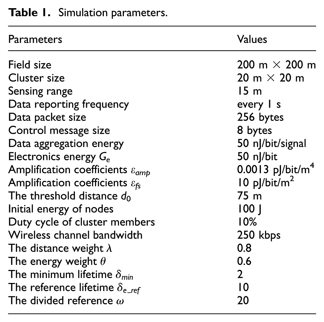
Due to the different possibilities in the target tracking scenarios, it is necessary to implement the simulation on the different conditions, such as the number of nodes and the maximum velocity of the target. For this work, five different node densities were considered, and the smallest node number was 500 and the largest was 3000. As a result, the simulation was allowed from sparse networks to highly dense networks, resulting in the performance comparison of the network scalability. Moreover, the coordinate of the sink was set to S₁(100, 100) or S₂(300, 100) in our network, which accorded with reality because sometimes the sink cannot be placed in the deployed area, such as battlefields and volcanic areas. In our simulation, the nodes could adjust the transmitting power according to the sending distance. The transmission cost between the nodes is evaluated by following equations^17,21

G_{Tx} (l, d) = {\begin{matrix} ({G_{Tx}}_{- e} + ε_{fs} * d^{α}) * l, d < d_{0} \\ ({G_{Tx}}_{- e} + ε_{amp} * d^{α}) * l, d \geq d_{0} \end{matrix}

(13)

G_{Rx} (k) = G_{Rx - e} * l

(14)

where G_Tx−e and G_Rx−e are the energy consumption by the radio electronics on circuit board; generally, the simulation parameters could be set as G_Tx−e= G_Rx−e = G_e. ε_fs and ε_amp (Joule/(bit mα)) are power amplification coefficients in two different channel models, respectively; they denote the power consumption transmitting a bit data under the condition of the required signal-to-noise ratio through a certain distance d. Moreover, $α$ ( $2 \leq α \leq 5$ ) is channel loss parameter which is determined by the transmission path characteristics. We set $α = 2$ , if $d < d_{0}$ while $α = 4$ , if $d \geq d_{0}$ , where $d_{0}$ is a distance threshold,^17,21 and l denotes the size of data packets. Moreover, we set T_min and T_max to be 10⁻³ and 0.1 s, respectively, T_ran ∈ (10⁻⁴, 10⁻⁵) s. In default scenarios, Table 1 shows a summary of the most relevant parameters for the simulations.

Table 1.

Simulation parameters.

Parameters	Values
Field size	200 m × 200 m
Cluster size	20 m × 20 m
Sensing range	15 m
Data reporting frequency	every 1 s
Data packet size	256 bytes
Control message size	8 bytes
Data aggregation energy	50 nJ/bit/signal
Electronics energy G_e	50 nJ/bit
Amplification coefficients ε_amp	0.0013 pJ/bit/m⁴
Amplification coefficients ε_fs	10 pJ/bit/m²
The threshold distance d₀	75 m
Initial energy of nodes	100 J
Duty cycle of cluster members	10%
Wireless channel bandwidth	250 kbps
The distance weight $λ$	0.8
The energy weight $θ$	0.6
The minimum lifetime $δ_{\min}$	2
The reference lifetime $δ_{e_ref}$	10
The divided reference $ω$	20

For a moving target, we assume a target in the sensing area moves continuously and randomly with a maximum acceleration a_max = 2 m/s² and the maximum velocity of the target changed from v_max = 5–30 m/s. This process model is given by

X_{k + 1} = [\begin{matrix} 1 & T & 0 & 0 \\ 0 & 1 & 0 & 0 \\ 0 & 0 & 1 & T \\ 0 & 0 & 0 & 1 \end{matrix}] X_{k} + [\begin{matrix} T^{2} / 2 \\ T \\ T^{2} / 2 \\ T \end{matrix}] v_{k}

(15)

where $X_{k} = [x, v_{x}, y, v_{y}]^{T}$ is the state of the moving target at k time instant; T is the sampling time interval, T = 1 s; $x, v_{x}$ are the position and velocity of the target in the direction of x-axis, respectively; $y, v_{y}$ are the position and velocity of the target in the direction of y-axis, respectively; $v_{k}$ is the state transition noise of the target, $v_{k} ~ N (0, σ)$ , and $σ = 2 \circ$ . In addition, the observation model is

Z_{k + 1} = H X_{k + 1} + w_{k + 1}, H = [\begin{matrix} 1 & 0 & 0 & 0 \\ 0 & 1 & 0 & 0 \\ 0 & 0 & 1 & 0 \\ 0 & 0 & 0 & 1 \end{matrix}]

(16)

where H is the observation matrix and $w_{k + 1}$ is the measurement noise which is assumed to be white Gaussian noise sequence with zero mean and the variance $σ$ . This scenario can represent the generalization of the target tracking problem.

The idle and sleep power consumption of sensor nodes, based on the real radio model of Texas Instruments CC1000, are 22.2 and 0.0006 mW, respectively, and the transition cost and delay between the sensor nodes states is shown in Table 2, where the cost and delay time to switch from column state to row state.

Table 2.

Transition power and delay (mW/ms).

Node state	Active (Tx)	Idle (Rx)	Sleep
Idle (Rx)	22.2/0.01	/	22.2/0.2
Sleep	0.5/0.05	0.5/0.05	/

Simulation results

The AEC comparison

First, we evaluate the proposed ETTA with two different sink locations to investigate its adaptability to the location of the sink. We set the maximum velocity of the target is 10 m/s and the number of sensor nodes is 1500. The results in Figures 6 and 7 show that the AEC variations of the approaches in our simulation. In Figures 6 and 7, the sinks are located at S₁ and S₂, respectively. Clearly, the AEC tends to increase as time goes on for all the approaches since the node needs to wake up for tracking mission and transmit the sensed data. From the results, we can see that ETTA can conserve at least 25% power than that in DARAL and CHSRDR approaches because the CH in ETTA has the most high energy efficiency. Moreover, the sensed data could be aggregated at CCH to avoid long-distance data transmitting so that the energy is further saved in ETTA. Unfortunately, in CHSRDR and LEACH, the CH just plays a role of manager and has lower energy efficiency, and other nodes have to be active for detecting. And each CH in LEACH sends the sensed data to the sink by one hop, which results in the long-distance transmission of large amounts of data. Since DARAL adopts the dynamic hierarchical cluster structure to transmit the sensed data so that it performs better than CHSRDR, especially when the sink is far away from the network.

Figure 6.

The AEC comparison when the sink was located at S₁.

Figure 7.

The AEC comparison when the sink was located at S₂.

Comparing the results in Figures 6 and 7, we can see that LEACH and CHSRDR perform better when the sink located at S₁ because they has the single-hop cluster communication and the far sink could especially lead to a lot of data packets transmitted by long distance. Although DARAL converts the long-distance data transmitting to the relative short distance transmitting by the hierarchical clusters, it cannot avoid that the sensed data from a target are sent to the sink through different routings so that the sensed data cannot be aggregated efficiently. In any case, the nodes in ETTA consume the least energy compared with other protocols in both sink locations. The advantages of ETTA are more obvious if the sink is far away from networks.

Second, we simulated the above-mentioned approaches under the different target maximum velocities. Figure 8 shows the AECs of the nodes for LEACH, CHSRDR, DARAL and ETTA after 600 s simulation time under six target velocities. Although the AEC on each node increases as the target velocity increasing, ETTA still outperforms the other approaches and has more efficient energy utility. From Figure 8, it is denoted that the performance of ETTA had a little reduction with the higher target velocity since it needs to select CCH more frequently than that with the lower target velocity. In CHSRDR, the CH discovery process needs to be executed frequently when the target has higher velocity so that the nodes consume more energy than that when the target has lower velocity. Also, the nodes in DARAL consume more energy when the target velocity increases due to the frequent hierarchical cluster forming. Since LEACH adopts the same principles for different target velocities, the energy consumptions almost does not vary with the target velocity.

Figure 8.

The AEC comparison under the different target velocities.

Finally, we further investigated the performance of the simulated approaches as the number of nodes changes while keeping the other parameters constant. Obviously, the AEC decreases with the increasing nodes, as shown in Figure 9, because only a CH is always awake in each cluster in clustered network structure. If node density increases, more sensor nodes could go to sleep status in the most of the simulation time, which results in further energy saving. As a result, higher node density can prolong the network lifetime.

Figure 9.

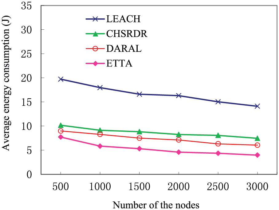
The AEC comparison under the different numbers of the nodes.

From Figure 9, we can see that ETTA consumes significantly less energy compared to LEACH, CHSRDR and DARAL. By considering the application constrains during CHs selection and data transmission process, ETTA saves more energy compared with the other approaches. Compared with LEACH, less long-distance data transmissions are required by the CHSRDR and DARAL due to the multi-hop transmitting among the CHs. However, since DARAL can organize sensors into more reasonable clusters, it achieves even higher energy efficiency compared with the CHSRDR.

The ATD comparison

Figure 10 illustrates the ATD changed with the target maximum velocities of different approaches. As a fixed reporting period is used, the ATD has little changes with the varied target velocities in all the approaches, because that there are always CHs in active mode to transmit data and the number of the data is almost the same under different target velocities. The sensed data in LEACH are directly sent to the sink by CHs without transmitted relay. As a result, LEACH achieves better real-time performance compared with the others. From Figure 10, we can see CHSRDR approach has the longest ATD value since it needs to execute the procedure of CH selection each time and consider the data recovery inside the network. The delay is shorter in DARAL than that in CHSRDR because DARAL built the hierarchical CHs dynamically and the CH could directly send the received data to its higher level CH rather than finding the next hop node. ETTA performs better than CHSRDR because the CHs in data transmitting chain keep active and each CH has an adaptive lifetime for data collection instead of selecting CH in every round. When the velocity of the target increased, the delay of ETTA changed a little longer since the CCH needs to be selected more frequently; nevertheless, ETTA has almost the same ATD value as DARAL.

Figure 10.

The ATD with different target velocities.

In Figure 11, we investigated the ATD changed with the number of the sensor nodes. We can see that if the other parameters are fixed, the average delay increases when node density increases. More nodes will be awake and detect the target at a higher density, which may create more data packets and hence increase the delivery delay. LEACH still has the lowest ATD compared with the other approaches for all node densities. When the node density increased, the ATD in CHSRDR and DARAL became longer since more sensed data need to be sent from different routings and each node has to decide who is the next hop in the hierarchical data transmitting structure. The delay is shorter in ETTA than that in the others because the data could be sent along the data transmitting chain. On the other hand, CCH can make data aggregation to reduce the number of transmission packets.

Figure 11.

The ATD with different numbers of detecting nodes.

The TSR comparison

Figure 12 shows the TSR changed with the target velocities. When the target velocity increased, the nodes in all the approaches had less time to respond for the appeared target. Sometimes, nodes had not enough time to be woken so that the TSR slightly decreased. However, all the approaches could nearly achieve 95% successful rate. Also, ETTA achieves satisfactory performance. Since the CH located at the edge of the cluster for target monitoring, ETTA almost have a stable performance in higher target velocity tracking. The simulation results indicate that LEACH has the lowest tracking error because all the sensed data are sent to the sink to achieve high accuracy regardless of the data aggregation.

Figure 12.

The TSR with different target velocities.

Figure 13 shows the TSR changed with the number of sensor nodes. We can see that the tracking performance was improved as the sensor nodes increased since more nodes detected the target with a higher node density and more sensed data were sent to the sink. However, when the number of nodes is more enough, increasing nodes density did not improve the TSR value. Inversely, overfull nodes can cause a lot of data collision to reduce the tracking performance. From Figure 13, we can see that all the approaches could achieve satisfactory successful rate if we selected a reasonable node density.

Figure 13.

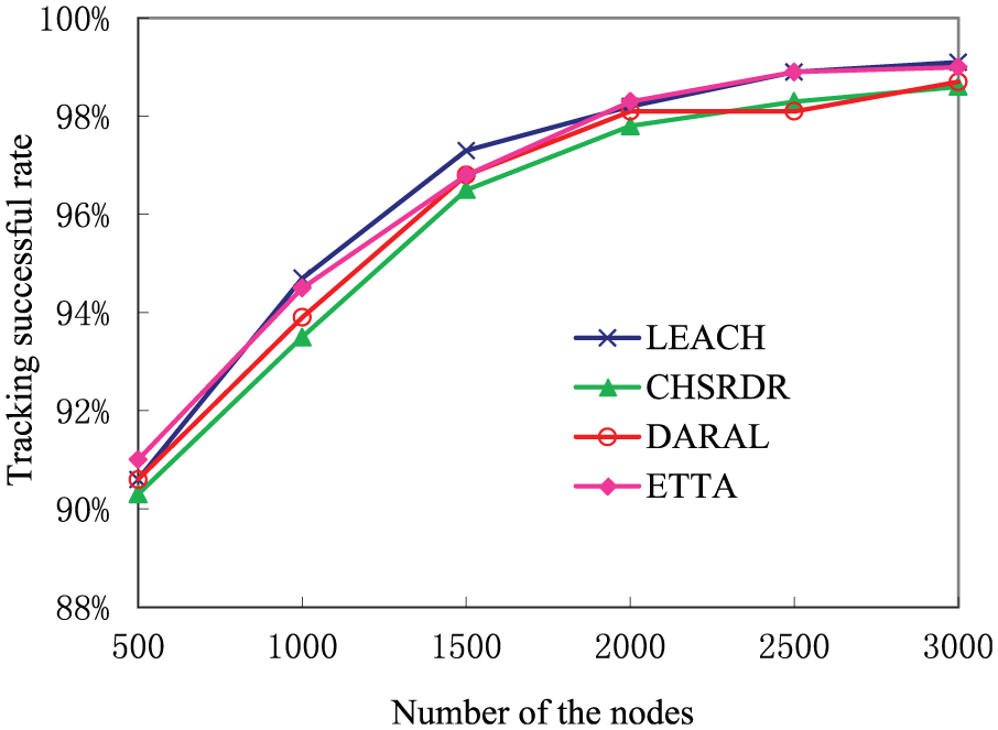
The TSR with different numbers of detecting nodes.

The NLS comparison

The results in Figures 14 and 15 show that the percentage of live nodes changed with the simulation time in the approaches. The sink in Figures 14 and 15 located at S₁ and S₂, respectively. In Figure 14, since the vast of nodes exhausted their energy after 2000 s while the residual nodes had to maintain the network connection and send the sensed data to the sink. Thus, there was a significant decrease of the percentage of live nodes after 2000 s. The percentage of live nodes in CHSRDR and DARAL was higher than that in LEACH since they adopted the multi-hop data transmitting among CHs. LEACH had the lowest percentage of live nodes because there were a lot of long-distance data transmissions from CHs to the sink. Nevertheless, each CH in ETTA located at the cluster edge and CCH could aggregate the sensed data near to the data source so that long-distance transmissions were reduced to the greatest extent. Consequently, ETTA could achieve high percentage of live nodes.

Figure 14.

The percentage of live node when the sink was located at S₁.

Figure 15.

The percentage of live node when the sink was located at S₂.

Compared to Figures 14 and 15, we also discover that when the sink is near to the network, LEACH and CHSRDR achieve better results than that when the sink is far away from the network. This is obviously due to the long-distance data transmitting from CHs to the sink. Taking the advantage of multi-hop data reporting strategies, the CHSRDR has more living nodes than LEACH. Due to the flexible hierarchical cluster scheme, DARAL achieves higher percentage of live nodes than LEACH and CHSRDR. The results in Figure 15 show that our method achieves better performance even in the networks located far away from the sink because a fewer data packets need to be sent from CHs to the sink and the CHs located at the edge of clusters so as to have high energy efficiency.

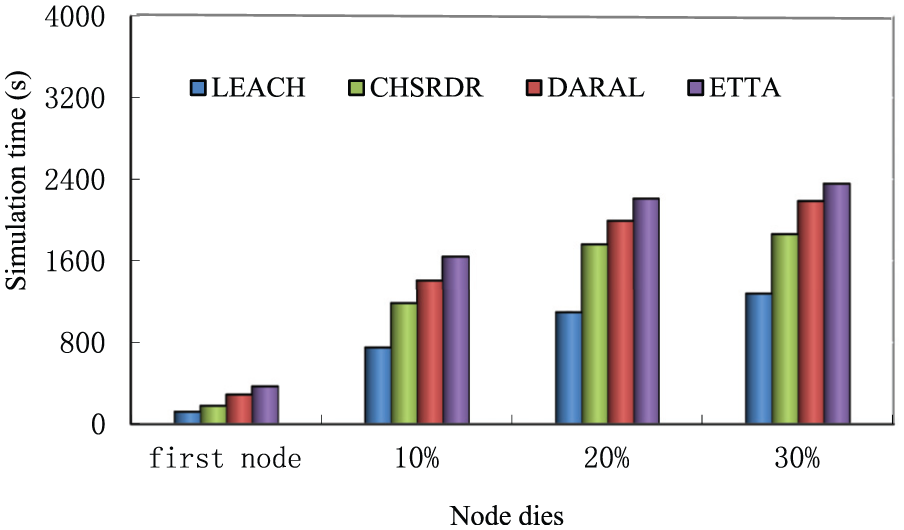
Figures 16 and 17 illustrate the network lifetime comparison of the different approaches for different percentages of the dead nodes, and the sink in Figures 16 and 17 located at S₁ and S₂, respectively. As shown, ETTA can significantly prolong the network lifetime in all cases. For example, if the lifetime is defined as the time when 20% of nodes die, ETTA achieves lifetime extensions by 28% and 20% compared to CHSRDR and DARAL when the sink located at S₁, and 30% and 15% when the sink located at S₂. Similar lifetime extensions are achieved for the other cases. This is caused by the following reason: (1) ETTA reduces the frequency of reconstructing clusters and balances energy consumption in the whole network since it allows each node to take the role of CH different times based on the residual energy of the node. (2) ETTA reduces the number of the active nodes because the CHs can play the roles of both manager and monitoring node. (3) ETTA adopts CCH to collect the sensed data so that it avoids transmitting large amounts of data through long distances.

Figure 16.

The NLS comparison when the sink was located at S₁.

Figure 17.

The NLS comparison when the sink was located at S₂.

From Figures 16 and 17, we can see that ETTA achieves a prolonged network lifetime in both cases, compared with LEACH, CHSRDR and DARAL. In a word, ETTA can decrease energy consumption and extend the lifetime span of target tracking WSNs without degrading the system performance.

Table 3 shows the average time for clustering setup in the different approaches. Obviously, the more computational complexity the clustering algorithm has, the longer time is cost in clustering setup stage. Both LEACH and ETTA are built clusters by the generated random digits in each node so that they have lower computational complexity than that in CHSRDR and DARAL. As a result, the average time of clustering setup in LEACH and ETTA is shorter than that in the other two algorithms. ETTA has longer clustering setup time than LEACH has because the nodes in ETTA need to wait a time period for CHs election. However, the waiting time can be controlled within a certain and reasonable range. Therefore, our ETTA also has good performance. Since CHSRDR has more complexity network structure and computational clustering algorithm, it costs longer clustering setup time. Due to building the hierarchical cluster structure, DARAL needs the longest clustering setup time.

Table 3.

Comparison of the average time for clustering setup in the different approaches.

Time	Approaches
Time	LEACH	CHSRDR	DARAL	ETTA
Average time for clustering setup (s)	0.236	0.492	0.683	0.315

LEACH: low-energy adaptive clustering hierarchy; ETTA: efficient target tracking approach.

Figure 18 shows the total number of data packets transmitted by the four approaches during target tracking. For all the data packets, every time one packet is sent, a data packet transmitting is counted. It can be seen that ETTA can reduce the total number of data packets transmitted in the network, compared to CHSRDR and DARAL approaches, because the data sensed from one target can be efficiently aggregated at CCH in ETTA, while the sensed data, which come from one target and have the strong correlations, are sent through different routings by CHs in the CHSRDR and DARAL approaches. The amount of data packets in LEACH is smaller than that in others, because every CH directly sends its data to the sink so as to reduce the relay data. Nevertheless, long-distance transmission of data consumes more energy and leads to exhausted CH. This way causes unbalanced energy consumption and frequent cluster structure reforming.

Figure 18.

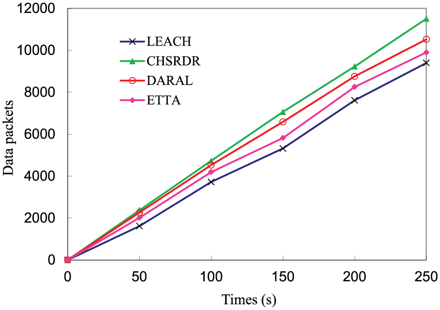
The data packets comparison during target tracking.

Conclusion

This article proposed an ETTA in sensor networks. ETTA combines the target tracking and cluster network structure. It can improve the energy efficiency of CHs and reduce energy consumption of data transmitting so as to extend network lifetime without debasing the system performance. ETTA is better than the other methods because CHs serve as both managers and monitoring nodes so that the other nodes can sleep more. Besides, each node takes the role of CH different times based on the residual energy so that the energy consumption is balanced in the whole network. Furthermore, CCH is used to collect the sensed data; hence, the data are aggregated near to the data source and the transmitting data are decreased. Our experiments proved that ETTA outperformed the state-of-the-art approaches by improving the energy consumption as well as prolonging the network lifetime by about 20% as the 20% nodes die.

Footnotes

Handling Editor: Zhi-Bo Yang

Declaration of conflicting interests

The author(s) declared no potential conflicts of interest with respect to the research, authorship, and/or publication of this article.

Funding

The author(s) disclosed receipt of the following financial support for the research, authorship, and/or publication of this article: This work was supported by the National Natural Science Foundation of China under grants 61601352, 6167 1356 and 61704127, the Fundamental Research Funds for the Central Universities under grant 20103176399, and the foundation of State Key Laboratory of Air Traffic Management system and Technology under grant SKLATM201702.

References

Yang

Radzienski

Kudela

et al . Two-dimensional modal curvature estimation via Fourier spectral method for damage detection. Compos Struct 2016; 148: 155–167.

Ding

et al . Sparsity-based algorithm for detecting faults in rotating machines. Mech Syst Signal Pr 2016; 72–73: 46–64.

Xiang

Lei

Wang

et al . Structural dynamical monitoring and fault diagnosis. Shock Vib 2015; 2015: 193831.

Ding

et al . Repetitive transients extraction algorithm for detecting bearing faults. Mech Syst Signal Pr 2017; 84: 227–244.

Mahmood

Seah

WKG

Welch

. Reliability in wireless sensor networks: a survey and challenges ahead. Comput Netw 2015; 79: 166–187.

Warrier

Kumar

Energy efficient routing in wireless sensor networks: a survey. In: Proceedings of the international conference on wireless communications, signal processing and networking, Chennai, India, 23–25 March 2016, pp.1987–1992. New York: IEEE.

Yang

Z-B

Chen

X-F

Xie

et al . The hybrid multivariate analysis method for damage detection. Struct Control Hlth 2016; 23(1): 123–143.

Sucasas

Radwan

Marques

et al . A survey on clustering techniques for cooperative wireless networks. Ad Hoc Netw 2016; 47(C): 53–81.

Lee

. A clustering algorithm based on mobility properties in mobile ad hoc networks. Int J Distrib Sens N 2015; 2015: 1–15.

10.

Heinzelman

Chandrakasan

Balakrishnan

. Energy-efficient communication protocol for wireless microsensor networks. In: Proceedings of the 33rd annual Hawaii international conference on system sciences, Maui, HI, 7 January 2000. New York: IEEE.

11.

Hosen

ASMS

Kim

Cho

. An energy efficient cluster formation and maintenance scheme for wireless sensor networks. J Inf Commun Converg Eng 2012; 10(3): 276–283.

12.

Younis

Fahmy

. HEED: a hybrid, energy-efficient, distributed clustering approach for ad hoc sensor networks. IEEE T Mobile Comput 2004; 3(4): 366–379.

13.

Gupta

Pandey

. An improved energy aware distributed unequal clustering protocol for heterogeneous wireless sensor networks. Eng Sci Technol Int J 2016; 19(2): 1050–1058.

14.

Singh

Goudar

Pant

et al . Cluster head selection by randomness with data recovery in WSN. Comput Sci Inf Technol 2014; 2(2): 97–107.

15.

Zhang

Pan

Liu

et al . A hybrid approach using mobile element and hierarchical clustering for data collection in WSNs. In: Proceedings of the wireless communications and networking conference, New Orleans, LA, 9–12 March 2015, pp.1566–1571. New York: IEEE.

16.

Abid

Nguyen

Seba

. New data aggregation approach for time-constrained wireless sensor networks. J Supercomput 2015; 71(5): 1678–1693.

17.

Chang

Tang

Cheng

et al . Dynamic hierarchical energy-efficient method based on combinatorial optimization for wireless sensor networks. Sensors 2017; 17(7): E1665.

18.

Estévez

Glösekötter

González

. DARAL: a dynamic and adaptive routing algorithm for wireless sensor networks. Sensors 2016; 16(7): 960.

19.

National ICT Australia–Castalia, https://github.com/boulis/Castalia

20.

OMNeT++ network simulator, http://www.omnetpp.org/

21.

Ren