A wireless sensor data-based coal mine gas monitoring algorithm with least squares support vector machines optimized by swarm intelligence techniques

Abstract

As the integral part of the new generation of information technology, the Internet of things significantly accelerates the intelligent sensing and data fusion in different industrial processes including mining, assisting people to make appropriate decision. These days, an increasing number of coal mine disasters pose a serious threat to people’s lives and property especially in several developing countries. In order to assess the risks arisen from gas explosion or gas poisoning, wireless sensor data should be processed and classified efficiently. Due to the fact that the “negative samples” of coal mine safety data are scarce, least squares support vector machine is introduced to deal with this problem. In addition, several swarm intelligence techniques such as particle swarm optimization, artificial bee colony algorithm, and genetic algorithm are applied to optimize the hyper parameters of least squares support vector machine. Using the popular deep neural networks, convolutional neural network and long short-term memory model, as comparisons, a number of experiments are carried out on several UCI machine learning datasets with different features. Experimental results show that least squares support vector machine optimized by swarm intelligence techniques can effectively handle classification task on different datasets especially on those datasets with limited samples and mixed attributes. The application of least squares support vector machine optimized by swarm intelligence techniques on real coal mine data demonstrates that this algorithm can process the data accurately and timely, therefore can warn of the accidents early in mining workplace.

Introduction

Although clean energy has been universally promoted in recent years, coal is still important energy in almost all developing countries. Even in developed countries, coal resource also plays an important role in industrial production and people’s daily life. For example, as released from Energy Information Administration (EIA), coal is the single largest primary energy for electricity generation in the United States during the first half of 2017. ¹ It is reasonable to say that coal mining will continue in a long period. In the mining workplace, a huge number of accidents are arisen from gas explosion or gas poisoning which pose serious threats to people’s life and properties. In order to prevent coal mine disasters and have a good use of sensor data, researchers all around the world have carried out several valuable works such as designing accurate chemical or electrical sensors, ² building effective wireless sensor networks, ³ and developing efficient online machine learning algorithms so as to deal with wireless sensor data appropriately and bridge the gap between cyber world and physical world in “intellimine system.” ⁴

Wireless sensor data processing is the key task to monitor gas composition and evaluate the safety status in mining workplace. ⁵ In the current decade, although deep learning models such as convolutional neural networks (CNN) ⁶ and recurrent neural networks (RNN) ⁷ show strong ability in image classification, ⁸ text processing, ⁹ and speech recognition ¹⁰ areas, they still have a lot of room to improve in risk assessment task. On one hand, deep learning is “data-thirsty.” Sometimes, deep neural networks need thousands of labeled samples in one task while the negative samples about coal mine safety situation, mine disasters, must be small and limited. On the other hand, we need fast response speed in this scenario but the computation time of deep neural networks is relatively long.^11,12 We hold the opinion that classic algorithms represented by support vector machine (SVM), ¹³ least squares support vector machine (LSSVM), ¹⁴ and Bayesian Classifier ¹⁵ are more suitable and effective for risk assessment on the condition that mining background can be perceived comprehensively. Generally, deep learning can fulfill this assignment. For example, CNN can be used to recognize the damage type in workplace; time series acquired by different sensors (especially gas sensors) can be analyzed by RNN effectively.

SVM is one of the most popular statistical learning methods. Different from neural networks which use multiple hidden layers to fit non-liner system, SVMs utilize kernel trick.^16,17 The implementation of SVM is based on the idea of finding the “max margin” and follows the structural risk minimization principle. ¹³ In order to improve the performance of SVM, scholars proposed various developed structures such as combining SVM with fuzzy control ¹⁸ and ensemble learning. ¹⁹ LSSVM is the main variant of SVM. In LSSVM, the loss function is improved using the quadratic terms of errors and the inequality constraints are replaced by the equality constraints. ¹⁴ The calculation process of LSSVM is relatively simple and fast so it is more suitable for coal mine gas monitoring task.

For algorithms like SVM and LSSVM, the selection of hyper parameters directly impacts algorithms’ performance. Sometimes, engineers need to have a good understanding of the data and determine parameters for the classifiers by experience. Normally, this manual method is time-consuming, experience dependent, and cannot achieve the optimal parameters. How to use intelligent optimization algorithms to choose suitable parameters has long been a research hot spot. YS Ji proposed a scheme based on ensemble Kalman filter which can optimize the characters and parameters of SVM; ²⁰ XF Yuan applied chaos algorithm to achieve the parameters of SVM for function approximation. ²¹ As the main optimization approach, evolutionary computation techniques such as genetic algorithm (GA) ²² and differential evolution (DE) algorithm, ²³ or more broadly defined, ant colony optimization (ACO), ²⁴ artificial bee colony (ABC) algorithm, ²⁵ artificial fish-swarm (AF) algorithm, ²⁶ artificial immune (AI) algorithm, ²⁷ and particle swarm optimization (PSO) ²⁸ are widely used in different tasks. These swarm intelligence algorithms are inspired by natural phenomena and biological behaviors. The “colonies” in algorithms can update appropriately through the evolution from one generation to another, therefore can find the optimal solution gradually. As a result, swarm intelligence algorithms are always employed to optimize parameters and select effective attributes for SVM and LSSVM. This hybrid strategy has been widely utilized in pattern recognition, ²⁹ fault diagnosis, ³⁰ and other detecting or forecasting works.^31,32

In this article, we try to introduce three classic swarm intelligence algorithms, GA, PSO, and ABC, to determine the parameters of LSSVM so as to enhance its learning ability. CNN ⁶ and a special kind of RNN, long short-term memory (LSTM), ³³ are used as comparisons to evaluate the performance of different models in different datasets. The article is organized as follows. In section “Background,” related work such as SVM, LSSVM, GA, PSO, and ABC are briefly explained. In section “LSSVM optimized by swarm intelligence techniques: SI-LSSVM,” LSSVM optimized by different evolutionary computation techniques (SI-LSSVM), together with deep learning models, are employed to solve several public classification tasks. Experiments about typical coal mine gas data are presented in section “Gas monitoring based on SI-LSSVM.” The conclusion is given in section “Conclusion.”

Background

SVM and LSSVM

Fundamentals

SVM is initially designed to deal with binary classification tasks. For a typical binary classification problem on the dataset $D=\{({\mathit{x}}_1,y_1),({\mathit{x}}_2,y_2),\dots ,({\mathit{x}}_n,y_n)\},y\in \{-1,1\}$ , the classifier could be a line in two-dimensional (2D) space, a plane in three-dimensional (3D) space, or a hyper-plane in high-dimensional feature space. In this space, SVM aims to find the “maximum margin.” We assume the expression of this hyper-plane is formula (1)

$${\mathit{\omega }}^{\mathrm{T}}\mathit{X}+b=0$$

$$\mathit{w}=({\mathit{w}}_1;{\mathit{w}}_2;\dots ;w_n)$$

(1)

where $\mathit{\omega }$ is a normal vector and $\mathit{b}$ is the displacement.

Ideally, this hyper-plane can classify samples correctly as equation (2)

$$\{\begin{array}{c}{\mathit{\omega }}^{\mathrm{T}}{\mathit{x}}_i+b\ge 1,y_i=1\hfill \\ \multicolumn{1}{c}{{\mathit{\omega }}^{\mathrm{T}}{\mathit{x}}_i+b\le -1,y_i=-1}\end{array}$$

(2)

In order to make sure that this plane can implement the “maximum margin,” the basic mathematical form of SVM can be transfer into a constrained minimization problem as equation (3)

$$\underset{\mathit{w},b}{min}\frac{1}{2}\Vert w{\Vert }^2$$

$$\mathrm{s}.\mathrm{t}.y_i({\mathit{\omega }}^{\mathrm{T}}{\mathit{x}}_i+b)\ge 1,i=1,2,\dots ,n$$

(3)

Using Lagrange multiplier method, we can get the “dual problem” of equation (3). The Lagrange function can be written as equation (4)

$$\underset{\mathit{w},b,\mathit{a}}{min}L(\mathit{w},b,\mathit{\alpha })=\frac{1}{2}\Vert \mathit{w}{\Vert }^2+\sum _{i=1}^m{\mathbf{\alpha }}_{\mathbf{i}}(1-y_i({\mathit{\omega }}^{\mathrm{T}}{\mathit{x}}_i+b))$$

$$\mathrm{s}.\mathrm{t}.y_i({\mathit{\omega }}^{\mathrm{T}}{\mathit{x}}_i+b)\ge 1,i=1,2,\dots ,n$$

(4)

where $\mathit{\alpha }=({\alpha }_1;{\alpha }_1;\dots ;{\alpha }_n)$ .

Setting that the partial derivatives of equation (4) on $\mathit{\omega }$ and $b$ are 0, we can get equations (5) and (6)

$$w=\sum _{i=1}^n{\alpha }_i{y}_i{\mathit{x}}_i$$

(5)

$$\sum _{i=1}^n{\alpha }_i{y}_i=0$$

(6)

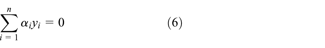
Then, the “dual problem” can be written as equation (7)

$$\underset{\alpha }{max}\sum _{i=1}^n{\alpha }_i-\frac{1}{2}\sum _{i=1}^n\sum _{j=1}^n{\alpha }_i{\alpha }_j{y}_i{y}_j{\mathit{x}}_i^{\mathrm{T}}{\mathit{x}}_j$$

$$\mathrm{s}.\mathrm{t}.\sum _{i=1}^n{\alpha }_i{y}_i=0$$

$${\alpha }_i\ge 0$$

(7)

where ${\alpha }_i$ is a Lagrange multiplier corresponding to a sample. Mostly, ${\alpha }_i=0$ . Only a few ${\alpha }_i\ne 0$ , the relative ${\mathit{x}}_i$ are those “support vectors.”

The expression of final classifier is equation (8)

$$f\left(x\right)=\mathrm{sgn}\left[({\mathit{\omega }}^{\mathrm{T}}\mathit{x}+b)\right]=\mathrm{sgn}(\sum _{i=1}^n{\alpha }_i{y}_i{\mathit{x}}_i^T\mathit{x}+b)$$

(8)

It should be mentioned that the derivation process above meets the Karush-Kuhn-Tucker (KKT) conditions. If we introduce the “soft margin” punishment factor C, the slack variable $\xi$ , and kernel function $\mathit{\phi }({\mathit{x}}_i)$ , the SVM model can be given as equation (9)

$$\underset{\mathit{w},b}{min}\frac{1}{2}\Vert \mathit{w}{\Vert }^2+C\sum _{i=1}^n{\xi }_i$$

$$\mathrm{s}.\mathrm{t}.y_i\left({\mathit{\omega }}^{\mathrm{T}}\mathit{\phi }\left({\mathit{x}}_i\right)+b\right)\ge 1-{\xi }_i,i=1,2,\dots ,n,{\xi }_i>0$$

(9)

Different from SVM, in LSSVM, inequality constraint is replaced by equation constraint and least-squares loss function is selected. The LSSVM model can be written as equation (10)

$$\underset{w,b}{min}\frac{1}{2}\Vert w{\Vert }^2+\frac{\mathrm{\gamma }}{2}\sum _{i=1}^n{e}_i^2$$

$$\mathrm{s}.\mathrm{t}.y_i={\mathit{\omega }}^{\mathrm{T}}\mathit{\phi }\left({\mathit{x}}_i\right)+b+e_i,i=1,2,\dots ,n$$

(10)

where $\mathrm{\gamma }$ is another writing style of “punishment factor,” and $e_i$ is the error of the model.

The major calculation methods of SVM or LSSVM include quadratic programming, sequential minimal optimization, and incremental strategy.

Classifiers for multi-class classification

Generally speaking, the sensor data about coal mine gas status can be classified into two groups: safe and dangerous. In special cases, we need to grade the mine into one of several security levels. In this situation, a multi-class classifier is needed. “One Vs Rest” method designed N classifiers for a multi-class task with N categories.^34,35 One category and others are classified by a binary classifier. Similar to “One Vs Rest,”“One Vs One” method trained $N(N-1)/2$ classifiers; one classifier can distinguish one category from another category among N categories respectively. ³⁶ Other strategies such as directed acyclic graph method ³⁷ and binary tree method ³⁸ can also transform SVM models.

Swarm intelligence techniques

Commonly, the main swarm intelligence algorithms can be divided into three types. The first kind of algorithms are based on evolutionary theory such as GA, DE, and AI. The population renew themselves by sharing information with each other. Another type of algorithms are represented by PSO. These algorithms, such as frog leaping algorithm and so on, search better solutions by the utilization of local information so as to upgrade the fitness. ABC is an improved algorithm with mixed features such as the local searching like PSO and the selection operation like GA. The last kind of algorithms, such as ACO, are not suitable for the optimization task for LSSVM. ACO has good performance in discrete and combinatorial optimization problems such as Traveling Salesman Problem, but it cannot deal with continuous numerical optimization tasks. Therefore, GA, PSO, and ABC are selected as the representatives in this article.

In evolutionary computation algorithms like PSO, ABC, and GA, one individual in the colony such as a bird, a chromosome, or a bee is relative to a solution of the problem to be optimized.^25,28 For instance, we can define an “N-dimensional particle” in PSO as a solution set, $(x_1,x_2,\dots ,x_n)$ , for a function optimization problem so as to find optimal solutions for the N-dimensional function, $f(x_1,x_2,\dots ,x_n)$ , by PSO. After the evolution of the population from one generation to the next, the algorithm can be close to the best solutions gradually.

PSO

The thinking of PSO derives from the special behavior of birds. In nature, the animals in a group can exchange their information about the environment and the food source. Each group of birds has a “leader” who is nearest to the food source. In one generation, all the birds in the group will follow the “leader” and search locally. If another bird gets a better position (closer to the food), this bird will become the new “leader.” In this way, those birds can move to the food finally.

We define the “particle,” also “the location of particle” as mentioned above. In addition, the “speed” of each particle also needs to be designed and calculated in PSO. At first, all the particles should be initialized in some ways such as random initialization or average initialization. Each particle has a “fitness” which is determined according to the optimization problem and can evaluate the quality of each particle. For the optimization problem aiming to search the minimum value for a function, the “fitness” can be designed as equation (11)

$$F\left(x_i\right)=\{\begin{array}{c}\frac{1}{1+f\left(x_i\right)}f\left(x_i\right)\ge 0\hfill \\ \multicolumn{1}{c}{1+\left|f\left(x_i\right)\right|f\left(x_i\right)<0}\end{array}$$

(11)

The speed of a particle determines its moving direction and displacement. In PSO, the speed can be calculated as equation (12)

$$v_{\mathrm{id}}(t+1)=\omega v_{\mathrm{id}}\left(t\right)+c_1{R}_1\left(t\right)(\mathrm{pbes}{t}_{\mathrm{id}}-x_{\mathrm{id}}\left(t\right))+c_2{R}_2\left(t\right)(\mathrm{gbes}{t}_d-x_{\mathrm{id}}\left(t\right))$$

(12)

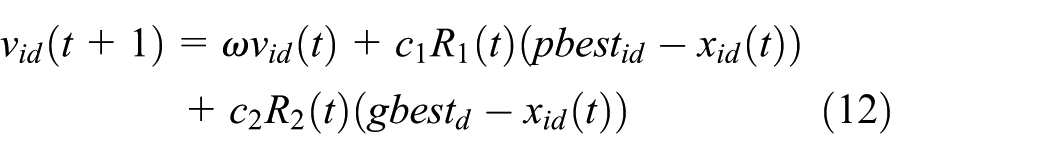
where v is the speed and x is the location of a particle; i is the serial number the particle; t is the serial number of the iteration; w is the inertia factor which illustrates the impact from the speed of the previous generation; $\mathrm{pbest}$ is the best location of the current particle (particle i); $\mathrm{gbest}$ is the global best location of the whole population; $c_1$ and $c_2$ are two constants which can balance the influence of two components; $R_1$ and $R_2$ are two random numbers; d = 1, 2, …, D; D is the dimension of particles.

After the speed is achieved, the new location of a particle can be computed as equation (13)

$$x_i(t+1)=x_i\left(t\right)+\varphi \left[v_i(t+1)\right]$$

(13)

where $\varphi$ is a limit function which can keep the speed of a particle in a reasonable range.

PSO can have a good use of valuable information both from the current individual and the whole colony. These days, PSO has already become one of the most popular optimization methods for its significant advantages such as simple algorithm structure and high robustness.

ABC

Similar to PSO, ABC is inspired by the biological behaviors of bees. The main development of ABC is that the bees are divided into different groups with different characters: the exploiting bees, the onlooker bees, and the scouters. The roles of bees can be changed by certain rules.

In ABC, each exploiting bee is correlated with a solution set, also a location of food source, as mentioned in the beginning of section “Swarm intelligence techniques.” Normally, the number of exploiting bees equals to the number of onlooker bees at the beginning. After initialization, the exploiting bees search locally as equation (14)

$$x_{\mathrm{id}}(t+1)=x_{\mathrm{id}}\left(t\right)+{\phi }_{\mathrm{id}}[x_{\mathrm{id}}\left(t\right)-x_{\mathrm{qd}}\left(t\right)]$$

(14)

where x is the location of food source; i is the serial number of the bee; d is one dimension in D dimensional solution set; t is the serial number of the iteration; ${\phi }_{\mathrm{id}}$ is a random number among [–1, 1]; q is randomly selected from [1, N] and $q\ne i$ ; N is the number of food source, also the number of exploiting bees.

To evaluate the quality of each bee, the “fitness” can be designed as equation (11). If one exploiting bee finds a better location, the older one will be replaced. According to the information, the quality of food source candidates, the onlooker bees will select candidates by a probability as equation (15). This method is also called roulette wheel selection method

$$p_i=\frac{F\left(x_i\right)}{\sum _{j=1}^{N}F\left(x_j\right)}$$

(15)

where $p_i$ is the profitability, $x_i$ is the location of the food source, and $F(x_i)$ is the fitness of $x_i$ .

The onlooker bees also search as equation (14). If one food source cannot be improved in continuous Limit iterations, the exploiting bee related to this food source will be changed into a scouter. In this situation, the food source is abandoned and the scouter search food as equation (16)

$$x_{\mathrm{id}}=x_d^{\min }+R_{\mathrm{id}}(x_d^{\max }-x_d^{\min })$$

(16)

where $x_d^{\min }$ is the minimal value on No. d dimension among all the bees and $x_d^{\max }$ is the maximum one; $R_{\mathrm{id}}$ is a random number between [0, 1]. Sometimes, we also initialize all the exploiting bees as equation (16) in the first period of algorithm.

GA

GA is the cornerstone of all the swarm intelligence algorithms. The optimization of GA follows the principle of “survival of the fittest” in natural selection. Different from PSO and ABC, ordinary GA utilizes binary coding strategy. Other coding strategies such as float coding are also very common. Generally speaking, GA consists of three operators: selection, crossover, and mutation.

The selection operator adopts the individuals with higher “fitness” as equation (11). Roulette wheel selection is also the most popular selection method in GA. Those individuals with higher fitness are more likely to copy their “gene” and join in the crossover process so as to keep their information in the next generation.

The aim of crossover operator is to combine the information from two different individuals so as to produce new and better offspring. According to the coding method, those two individuals will crossover with each other in different ways. Take the “binary coding” and “single point crossover” as the example. Normally, the matching individuals and crossover points are determined randomly. The crossover process can be illustrated as Table 1.

Table 1.

The crossover operator.

Number	Individual	Matching object	Crossover point	New individual
1	01100	3	3	01001
2	11000	4	5	11001
3	11001	1	3	11100
4	10011	2	5	10010

Gene mutation can introduce more randomness in the population. Mutation operator gives GA a possibility to find an individual with a higher fitness. The mutated individuals and the mutation points can be determined by some heuristic knowledge or just stochastically. The example of mutation process is shown in Table 2. In this example, we also use “binary mutation.”

Table 2.

The mutation operator.

Number	Individual	Mutation point	New individual
1	01100	3	01000
2	11000	5	11001
3	11001	3,5	11100
4	10011	5	10010

LSSVM optimized by swarm intelligence techniques: SI-LSSVM

Parameter optimization using PSO, ABC, and GA

Algorithm details

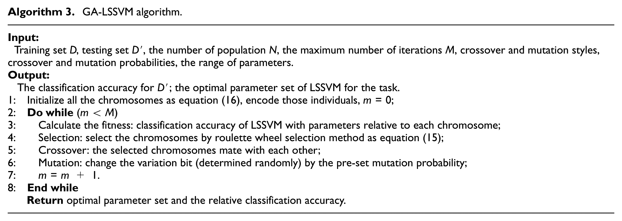
PSO-LSSVM, ABC-LSSVM, and GA-LSSVM algorithms can be written as Algorithms 1–3, respectively.

Algorithm 1. PSO-LSSVM.
Input:  Training set D, testing set D′, the number of population N, the maximum number of iterations M, the value of $c_1,c_2$ and w, the range of hyper parameters.
Output:
The classification accuracy for D′; the optimal parameter set for the task.
1: Initialize the location and speed of each particle as (16) and (20), m = 0;
2: Do while (m < M)
3:  Calculate the fitness: classification accuracy of LSSVM with parameters relative to the particle;
4:  Update pbest, gbest;
5:  Update the location and speed of each particle as (12) and (13);
6:  m = m + 1.
7: End while
Return optimal parameter set and the relative classification accuracy.

Algorithm 2. ABC-LSSVM algorithm.
Input:  Training set D, testing set D′, the number of population N, the maximum number of iterations M, the value of limit, the range of parameters.
Output:
The classification accuracy for D′; the optimal parameter set of LSSVM for the task.
1: Initialize the location of each exploiting bee as equation (16), m = 0;
2: Do while (m < M)
3:  Calculate the fitness: classification accuracy of LSSVM with parameters relative to each bee;
4:  If (the fitness of one bee cannot be improved in continuous Limit iteration), change this bee into scouts;
5:  The onlooker bees select their location by roulette wheel selection method as equation (15);
6:  The exploiting bees and onlooker bees update their location by equation (14);
7:  m = m + 1
8: End while
Return optimal parameter set and the relative classification accuracy.

Algorithm 3. GA-LSSVM algorithm.
Input:  Training set D, testing set D′, the number of population N, the maximum number of iterations M, crossover and mutation styles, crossover and mutation probabilities, the range of parameters.
Output:
The classification accuracy for D′; the optimal parameter set of LSSVM for the task.
1: Initialize all the chromosomes as equation (16), encode those individuals, m = 0;
2: Do while (m < M)
3:  Calculate the fitness: classification accuracy of LSSVM with parameters relative to each chromosome;
4:  Selection: select the chromosomes by roulette wheel selection method as equation (15);
5:  Crossover: the selected chromosomes mate with each other;
6:  Mutation: change the variation bit (determined randomly) by the pre-set mutation probability;
7:  m = m + 1.
8: End while
Return optimal parameter set and the relative classification accuracy.

Kernel experiments

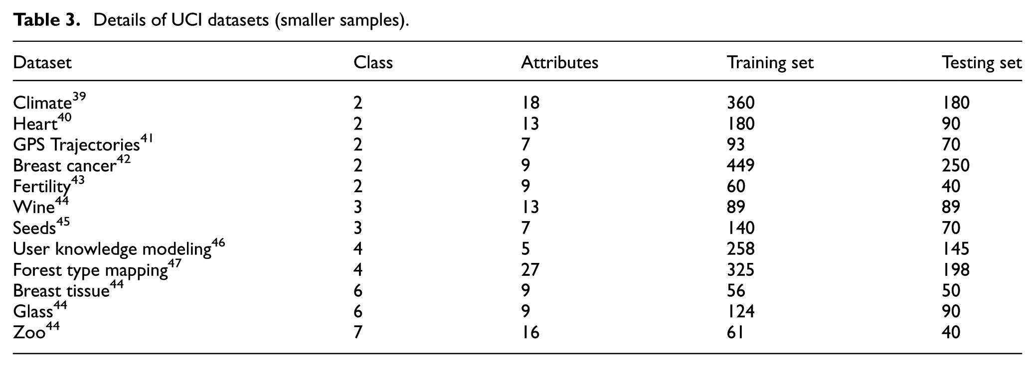
At first we carried out a group of experiments to evaluate different kernels for LSSVM: RBF kernel, linear kernel, and polynomial kernel. Heart, Wine, and Glass datasets (shown in Table 3) are taken as detailed examples. In PSO, $w$ is set at 0.6, $c_1$  =  $c_1$  = 2. In ABC, limit is set at 20. In GA, crossover probability is set at 0.6 and mutation probability is set at 0.01. Binary coding strategy with 20 bits is used in our GA for each hyper parameter. We adopt one-point crossover and one-point mutation strategies. For multi-class datasets, one-vs-one method is selected.

Table 3.

Details of UCI datasets (smaller samples).

Dataset	Class	Attributes	Training set	Testing set
Climate 39	2	18	360	180
Heart 40	2	13	180	90
GPS Trajectories 41	2	7	93	70
Breast cancer 42	2	9	449	250
Fertility 43	2	9	60	40
Wine 44	3	13	89	89
Seeds 45	3	7	140	70
User knowledge modeling 46	4	5	258	145
Forest type mapping 47	4	27	325	198
Breast tissue 44	6	9	56	50
Glass 44	6	9	124	90
Zoo 44	7	16	61	40

Since the performance of polynomial kernel is worst in cross-validation experiments as Table 4, we only compare SI-LSSVM models with RBF kernel (17) or linear kernel (18)

$$\mathit{\phi }\left({\mathit{x}}_i\right)=\mathbf{K}({\mathit{x}}_i,{\mathit{x}}_k)=\mathbf{exp}(-\frac{{\Vert {\mathit{x}}_i-{\mathit{x}}_k\Vert }^2}{{\sigma }^2})$$

(17)

$$\mathit{\phi }\left({\mathit{x}}_i\right)=\mathbf{K}({\mathit{x}}_i,{\mathit{x}}_k)={\mathit{x}}_{\mathit{i}}^{\mathit{T}}{\mathit{x}}_{\mathit{k}}$$

(18)

Table 4.

The performance of three kernels in cross-validation experiments.

Cross-validation	RBF	Linear	Poly
Heart	81.1	86.7	65.6
Wine	98.7	97.3	93.7
Glass	53.5	51.1	50

For this model optimization task, we adopt the accuracy of LSSVM as the fitness of swarm intelligence algorithms. In PSO and ABC, floating-point encoding method is selected, therefore the population can be defined as $\mathit{P}=({\mathit{p}}_1,{\mathit{p}}_2,\dots ,{\mathit{p}}_{\mathit{n}})$ . The individual ${\mathit{p}}_i$ in our models can be defined as a 2D vector for RBF kernel as shown in equation (19) or a variable, γ for linear kernel

$${\mathit{p}}_i=\{p_0,p_1\}=\{\mathrm{\gamma },{\sigma }^2\}$$

(19)

At the beginning, all the individuals can be initialized as equation (16). Samples can be normalized as equation (20)

$$x\prime =\frac{x-x_{\min }}{x_{\max }-x_{\min }}$$

(20)

Particularly, in GA, we use the classical binary encoding strategy. In GA-LSSVM, one individual can be encoded as a 2-line matrix with 0 and 1 for RBF kernel or a vector for linear kernel. Besides, in PSO, the speed of one individual can be initialized as equation (21)

$$v_i=R\times v_{\max }$$

(21)

where $R$ is a random number between [0,1] and $v_{\max }$ is the pre-set upper limit of the speed.

All the experiments are carried out nine times, the average accuracies are recorded in Table 5.

Table 5.

The performance of SI-LSSVM with different kernels.

UCI dataset	SI-LSSVM	RBF	Linear
Heart (Population = 4, Iteration = 10)	PSO-LSSVM	86.7	86.7
	ABC-LSSVM	86.6	86.7
	GA-LSSVM	86.3	86.7
Wine (Population = 4, Iteration = 25)	PSO-LSSVM	99.6	97.8
	ABC-LSSVM	99.0	97.5
	GA-LSSVM	98.9	96.6
Glass (Population = 6, Iteration = 50)	PSO-LSSVM	64.7	56.7
	ABC-LSSVM	64.4	55.6
	GA-LSSVM	64.4	55.7

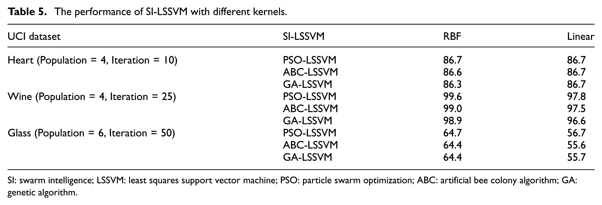
SI: swarm intelligence; LSSVM: least squares support vector machine; PSO: particle swarm optimization; ABC: artificial bee colony algorithm; GA: genetic algorithm.

As shown in Table 5, the performance of RBF kernel is similar to that of liner kernel in binary classification dataset. In multi-class classification tasks (Wine, Glass), PSO-LSSVM with RBF kernel can obtain the best accuracies and it is far better than that of liner kernel. Considering the experimental results comprehensively, SI-LSSVM (especially the PSO-LSSVM) with RBF kernel is the preferred model. In this article, we use RBF kernel (17) as kernel function $\mathit{\phi }({\mathit{x}}_i)$ in our LSSVM model, so γ and ${\sigma }^2$ are the parameters to be optimized.

Experiments on datasets with small samples

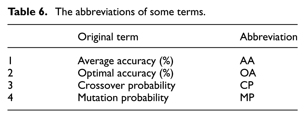
We use some abbreviations in the article as Table 6.

Table 6.

The abbreviations of some terms.

	Original term	Abbreviation
1	Average accuracy (%)	AA
2	Optimal accuracy (%)	OA
3	Crossover probability	CP
4	Mutation probability	MP

In this section, we use datasets with relatively small samples to evaluate the performance of SI-LSSVM models. The details of these datasets can be described in Table 5.

In this section, all the experiments are conducted on a PC with Intel core(TM) i5-5300U CPU @ 2.30 GHz processor and 8 GB RAM. Software developing environment is MATLAB R2016a on 64 bit windows 7 system.

Parameter determination experiments

It should be mentioned that the introduction of swarm intelligence algorithms will bring some new hyper parameters. We carried out several experiments to evaluate different parameter sets in PSO, ABC, and GA and then determine the appropriate parameters. Generally speaking, these parameters do not have very direct impacts to classification accuracy and they are relatively easy to adjust compared with those parameters in LSSVM. Since the population size is mainly relative to the complexity of the problem, we do not analyze it along with other parameters. Taking Heart, Wine, and Glass datasets as examples, statistical results are recorded in Table 7. In these experiments, we set the swarm size at 4 for Heart and Wine datasets and 10 for glass dataset.

Table 7.

Parameter determination of swarm intelligence algorithms.

Algorithm	Parameter set	Heart			Wine			Glass
		AA	OA	It	AA	OA	It	AA	OA	It
PSO-LSSVM	w, c 1, c2
	0.6, 2, 2	86.7	86.7	100	99.8	100	100	66.0	66.7	100
	0.4, 2, 2	86.7	86.7	100	99.8	100	100	64.8	65.6	100
	0.6, 1.5, 1.5	86.7	86.7	100	99.8	100	100	64.9	66.7	100
	0.3, 1.2, 1.2	86.7	86.7	100	99.6	100	100	64.6	65.6	100
	0.3, 0.5, 0.5	86.7	86.7	100	99.6	100	100	64.6	65.6	100
	0.1, 0.5, 0.5	86.7	86.7	100	99.6	100	100	64.4	64.4	100
	0.1, 0.1, 0.1	86.7	86.7	100	99.9	100	100	65.4	65.6	100
ABC-LSSVM	Limit
	3	86.7	86.7	100	99.3	100	100	64.7	66.7	100
	5	86.7	86.7	100	99.1	100	100	64.4	64.4	100
	10	86.7	86.7	100	99.1	100	100	64.7	66.7	100
	15	86.7	86.7	100	99.1	100	100	64.4	64.4	100
	20	86.7	86.7	100	99.4	100	100	64.8	65.6	100
GA-LSSVM	CP, MP
	0.4, 0.01	86.2	86.7	100	98.8	98.9	100	64.4	64.4	100
	0.4, 0.1	86.6	86.7	100	98.9	98.9	100	64.4	64.4	100
	0.6, 0.01	86.2	86.7	100	98.9	98.9	100	64.4	64.4	100
	0.6, 0.1	86.3	86.7	100	99.0	100	100	64.4	64.4	100
	0.8, 0.1	86.6	86.7	100	99.3	100	100	64.4	64.4	100

AA: average accuracy; OA: optimal accuracy; LSSVM: least squares support vector machine; PSO: particle swarm optimization; ABC: artificial bee colony; GA: genetic algorithm; CP: crossover probability; MP: mutation probability.

Bold values are those parameter sets with better performance and the relative accuracies.

As shown in Table 7, in binary classification tasks, GA-LSSVM is more parameter sensitive. PSO-LSSVM and ABC-LSSVM are more parameter sensitive in multi-class classification tasks.

Detailed comparative experiments

As detailed examples, the performances of SI-LSSVM models on Heart, Wine, and Glass datasets are listed in Tables 8–10, respectively. In our experiments, the hyper parameters of LSSVM, γ and ${\sigma }^2$ , are selected among [0.01, 300]. We use the parameters recorded in Table 4. Binary coding strategy with 20 bits is applied in our GA for each hyper parameter, so one chromosome is designed as a 2 × 20 matrix. We adopt “one-point” crossover and mutation strategies. For multi-class datasets, one-vs-one method is selected. ³⁶ In addition, cross-validation parameter determining method and manual method (determine the parameters by the experimenter) are also utilized in our experiments as comparisons. These experiments are carried out with different swarm sizes and iterations. We calculated average accuracy and time for a fixed parameter combination. Each group of experiments is repeated nine times.

Table 8.

Experimental results of algorithms on Heart dataset.

Heart	Population	It	Accuracy	$\mathbf{\gamma }$	${\mathbf{\sigma }}^2$	Training time	Testing time
PSO-LSSVM	20	300	86.7	289.3542	178.5996	127.4	1.55
	10	200	86.7	137.1477	120.9090	44.2	1.53
	10	100	86.7	1.09734	53.9377	23.1	1.52
	10	100	86.7	0.620666	29.4809	22.8	1.58
	6	100	86.7	2.35902	16.8497	12.4	1.52
	6	100	86.7	18.4533	299.7429	12.9	1.50
	4	50	86.7	270.818	191.613	6.1	1.48
	4	50	86.7	5.26196	167.628	5.2	1.52
	4	25	86.7	2.82254	125.21	3.4	1.56
	4	25	86.7	19.4952	300	3.1	1.52
Average accuracy and time (9 times)	4	25	86.7	–	–	3.26	1.52
	6	100	86.7	–	–	12.13	1.51
ABC-LSSVM	20	300	86.7	157.469	117.725	140.3	1.53
	10	200	86.7	126.87	129.31	45.1	1.51
	10	100	86.7	213.509	149.455	22.2	1.52
	10	100	86.7	186.0020	136.2204	22.7	1.58
	6	100	86.7	102.434	95.0986	13.6	1.61
	6	100	86.7	10.9608	159.9090	14.8	1.58
	4	50	86.7	113.018	107.607	5.2	1.56
	4	50	86.7	161.6023	120.6349	5.4	1.56
	4	25	85.6	300	272.124	3.2	1.52
	4	25	86.7	25.4065	26.8995	3.0	1.53
Average accuracy and time (9 times)	4	25	86.15	–	–	3.13	1.51
	6	100	86.7	–	–	13.2	1.55
GA-LSSVM	20	300	86.7	12.5981	179.601	115.8	1.61
	10	200	86.7	163.823	145.133	43.2	1.55
	10	100	86.7	233.363	145.216	21.6	1.52
	10	100	86.7	110.0268	105.6369	19.5	1.52
	6	100	86.7	76.3072	85.1124	12.4	1.48
	6	100	86.7	265.8345	193.3831	11.3	1.53
	4	50	86.7	6.52033	241.619	6.7	1.56
	4	50	86.7	229.588	174.94	6.7	1.54
	4	25	86.7	273.247	156.53	3.2	1.5
	4	25	85.6	93.2396	297.277	3.4	1.52
Average accuracy and time (9 times)	4	25	86.0	–	–	3.17	1.51
	6	100	86.7	–	–	11.9	1.53
Cross-validation	–	–	81.1	5.1102	1.2605	4.8	1.52
	–	–	81.1	5.9348	1.5999	4.1	1.52
Default parameters	–	–	82.2	10	10	1.7	1.62
	–	–	56.7	10	0.2	1.5	1.64

LSSVM: least squares support vector machine; PSO: particle swarm optimization; ABC: artificial bee colony; GA: genetic algorithm.

Table 9.

Experimental results of algorithms on Wine dataset.

Wine	Population	It	Accuracy	$\mathbf{\gamma }$	${\mathbf{\sigma }}^2$	Training time	Testing time
PSO-LSSVM	10	100	100	1.77362	18.3232	29.3	0.48
	10	100	100	1.056	15.0923	29.3	0.43
	6	100	100	2.44904	36.5938	16.9	0.50
	6	100	100	1.43774	10.6816	15.6	0.43
	4	50	100	5.00064	54.9659	5.8	0.39
	4	50	100	1.77527	21.7605	6.1	0.45
	4	50	100	2.73304	12.6362	5.6	0.45
	4	50	100	0.777642	9.71814	6.2	0.43
	4	25	100	4.90643	22.1601	3.5	0.49
Average accuracy and time (9 times)	4	50	100	–	–	6.26	1.52
	6	100	100	–	–	15.13	1.51
ABC-LSSVM	10	100	100	6.35958	67.2438	28.4	0.44
	10	100	98.9	122.531	44.1084	28.8	0.43
	6	100	98.9	125.74	144.158	16.8	0.39
	6	100	100	4.49727	37.7938	18.5	0.51
	4	50	98.9	62.38	156.349	6.4	0.43
	4	50	98.9	60.0541	203.9	6.9	0.45
	4	50	98.9	21.1986	165.051	6.7	0.46
	4	50	100	5.32209	51.6609	6.8	0.52
	4	25	98.9	148.7699	91.0530	3.7	0.44
Average accuracy and time (9 times)	4	50	99.18	–	–	6.43	1.51
	6	100	99.45	–	–	17.2	1.55
GA-LSSVM	10	100	98.9	12.8049	21.4435	26.2	0.48
	10	100	100	4.96513	56.762	25.1	0.46
	6	100	98.9	260.2	117.258	14.2	0.51
	6	100	100	6.58241	63.4071	14	0.44
	4	50	98.9	58.7755	129.519	6.4	0.47
	4	50	98.9	150.929	40.3929	6.8	0.52
	4	50	98.9	51.1216	292.103	7.1	0.40
	4	50	100	5.96559	63.8943	6.3	0.41
	4	25	98.9	18.5531	22.5155	3.5	0.42
Average accuracy and time (9 times)	4	50	99.18	–	–	6.17	1.51
	6	100	99.31	–	–	14.9	1.53
Cross-validation	–	–	98.9	38.8332	74.8296	2.9	0.40
	–	–	98.9	134.818	102.9182	2.3	0.45
Default parameters	–	–	98.9	135.0532	174.0753	2.4	0.42
	–	–	97.8	10	10	0.5	0.41

LSSVM: least squares support vector machine; PSO: particle swarm optimization; ABC: artificial bee colony; GA: genetic algorithm.

Table 10.

Experimental results of algorithms on Glass dataset.

Glass	Population	It	Accuracy	$\mathbf{\gamma }$	${\mathbf{\sigma }}^2$	Training time	Testing time
PSO-LSSVM	10	200	65.6	1.75969	23.432	156.7	0.58
	10	200	64.4	263.623	297.496	168.3	0.53
	10	200	65.6	2.54091	23.3694	155.2	0.50
	10	200	65.6	0.941973	10.2708	158.3	0.43
	10	100	64.4	296.295	291	88.1	0.59
	10	100	66.7	3.02245	26.5733	85.5	0.45
	10	100	66.7	2.89092	22.9878	77.6	0.49
	10	100	65.6	2.553	30.3676	81.7	0.43
	20	100	66.7	3.36432	26.9222	156.3	0.49
	20	100	66.7	3.15262	27.7584	160.3	0.48
	20	100	66.7	2.88749	25.5463	165.2	0.56
Average accuracy and time (9 times)	10	200	65.29	–	–	158.8	0.52
	10	100	65.86	–	–	83.2	0.51
ABC-LSSVM	10	200	64.4	216.982	187.593	154.1	0.49
	10	200	64.4	125.74	144.158	155.7	0.51
	10	200	64.4	123.845	148.179	152.3	0.43
	10	300	66.7	3.428	26.0226	233.5	0.55
	10	100	65.6	2.76284	22.3091	86.1	0.46
	10	100	65.6	0.747323	12.8223	81.3	0.52
	10	100	65.6	3.16233	19.8777	80.3	0.54
	20	100	64.4	189.674	184.753	165.5	0.40
	20	100	64.4	89.1077	121.2536	160.7	0.55
	20	100	64.4	221.2559	188.8784	164.5	0.52
Average accuracy and time (9 times)	10	200	64.4	–	–	153.4	0.48
	10	100	65.6	–	–	81.2	0.53
GA-LSSVM	10	200	64.4	19.9853	57.6663	151.4	0.51
	10	200	64.4	242.531	209.064	156	0.44
	10	200	64.4	54.9598	97.4756	158	0.47
	10	100	64.4	161.755	156.47	80	0.52
	10	100	64.4	227.484	191.069	71.9	0.50
	10	100	64.4	75.6237	114.093	75.8	0.41
	20	100	64.4	37.7748	74.4814	158.3	0.52
	20	100	64.4	148.291	160.642	159.5	0.44
	20	100	64.4	87.6637	122.181	161.2	0.53
Average accuracy and time (9 times)	10	200	64.4	–	–	155.6	0.49
	10	100	64.4	–	–	73.2	0.47
Cross-validation	–	–	52.2	6.6506	1.8025	7.2	0.55
	–	–	52.2	8.849	1.2048	7.4	0.42
Default parameters	–	–	52.2	7.4433	1.107	7.7	0.51
	–	–	55.6	10	10	0.5	0.49

LSSVM: least squares support vector machine; PSO: particle swarm optimization; ABC: artificial bee colony; GA: genetic algorithm.

As illustrated in Table 8 and Figure 1, on Heart dataset, all these three algorithms can achieve good classification accuracies. When population is 6 as Figure 2, ABC has a better performance than GA. If the swarm size is 4, PSO can find the parameters in a shorter time. In the LSSVM optimization task, PSO and ABC perform better than GA. All the SI algorithms obtain better solutions than cross-validation method and man-made method.

Figure 1.

Fitness curves of three algorithms on Heart dataset (best fitness in the median run of 9 runs).

Figure 2.

Fitness curves of three algorithms on Wine dataset (best fitness in the median run of 9 runs).

The training time of GA-LSSVM is shorter than other models. Compared with PSO, ABC needs more training time. There is no obvious difference in the testing time of three models.

SI-LSSVM performs best on wine dataset. These models can completely classify the samples correctly and have 100% accuracies. PSO optimizer also performs best and has a highest average accuracy, 100%. ABC has a similar performance to GA. As shown in Figure 3, PSO can get the optimal parameters quicker. In the limited training cycles, 50 cycles, this optimizer is more likely to have a good performance. In a longer training time, GA can also obtain the expected parameters.

Figure 3.

Fitness curves of three algorithms on Glass dataset (best fitness in the median run of 9 runs).

On this dataset, PSO even has a shorter training time than GA in one specific experiment. From the perspective of average training time, GA performs best. The training time of ABC is longer than that of PSO and GA.

As shown in Table 10 and Figure 3, on glass dataset, SI-based LSSVMs obtained the accuracies greater than 60%; while the accuracies gained by cross-validation method or man-made method are only more than 50%. Specifically, PSO-LSSVM gets the highest classification accuracy; ABC can also find those better parameters in a relatively long iteration (300 cycles). Similar to the experiments on other datasets, the training time of ABC is longer than that of PSO and GA.

Swarm size analysis

We also analyze the impact of swarm size to SI-LSSVM models. Experimental results on Wine and Glass datasets are illustrated in Figure 4. In PSO, w = 0.6, c₁ = 2, c₂ = 2; in ABC, limit = 20; in GA, CP = 0.8, MP = 0.1. All the iteration numbers are set at 100.

Figure 4.

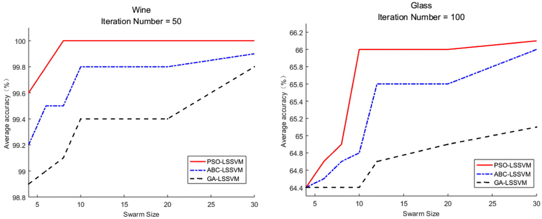
Fitness curves of three algorithms on Wine and Glass datasets with different swarm sizes.

Figure 4 shows the performance of these models with different swarm size. Obviously, the performance of all the models becomes better when swarm size is increased. For the SI-LSSVM model in this article, the increase in population will lengthen the running time proportionally. In some large scale datasets, time overhead would be huge. This is the reason why the comparative analysis on small swarm size is conducted in this article. If the computational resources are sufficient, larger swarm size can improve the classification ability of SI-LSSVM significantly. It should also be mentioned that although the training time of SI-based models is a little long, the testing time of these algorithms is around or even less than 1 s. This means that LSSVM model can react quickly in emergency.

Statistical results

Statistical results on 12 datasets are recorded in Tables 11–13.

Table 11.

The performance of PSO-LSSVM in different datasets.

Dataset	Parameter set (w, c1, c2)	AA	OA	Dataset	Parameter set (w, c1, c2)	AA	OA
Climate (Population = 4, Iteration = 20)	0.6, 2, 2	93.9	93.9	Seeds (Population = 4, Iteration = 30)	0.6, 2, 2	90	90
	0.1, 0.5, 0.5	93.9	93.9		0.1, 0.5, 0.5	89.8	90
Heart (Population = 4, Iteration = 20)	0.6, 2, 2	86.7	86.9	User modeling (Population = 4, Iteration = 30)	0.6, 2, 2	89.5	89.7
	0.1, 0.5, 0.5	86.7	86.7		0.1, 0.5, 0.5	89.4	89.7
GPS Trajectories (Population = 4, Iteration = 20)	0.6, 2, 2	95.7	95.7	Forest (Population = 4, Iteration = 30)	0.6, 2, 2	91.9	91.9
	0.1, 0.1, 0.1	95.5	95.7		0.1, 0.5, 0.5	91.7	91.9
Breast cancer (Population = 4, Iteration = 30)	0.6, 2, 2	97.6	98	Breast tissue (Population = 4, Iteration = 10)	0.6, 2, 2	69.3	72
	0.1, 0.5, 0.5	97.4	97.6		0.1, 0.5, 0.5	70	72
Fertility (Population = 4, Iteration = 10)	0.6, 2, 2	92.2	92.5	Glass (Population = 10, Iteration = 100)	0.6, 2, 2	66.0	66.7
	0.1, 0.5, 0.5	91.4	92.5		0.1, 0.5, 0.5	64.4	64.4
Wine (Population = 4, Iteration = 30)	0.6, 2, 2	99.8	100	Zoo (Population = 4, Iteration = 10)	0.6, 2, 2	92.5	92.5
	0.1, 0.5, 0.5	99.6	100		0.1, 0.5, 0.5	92.5	92.5

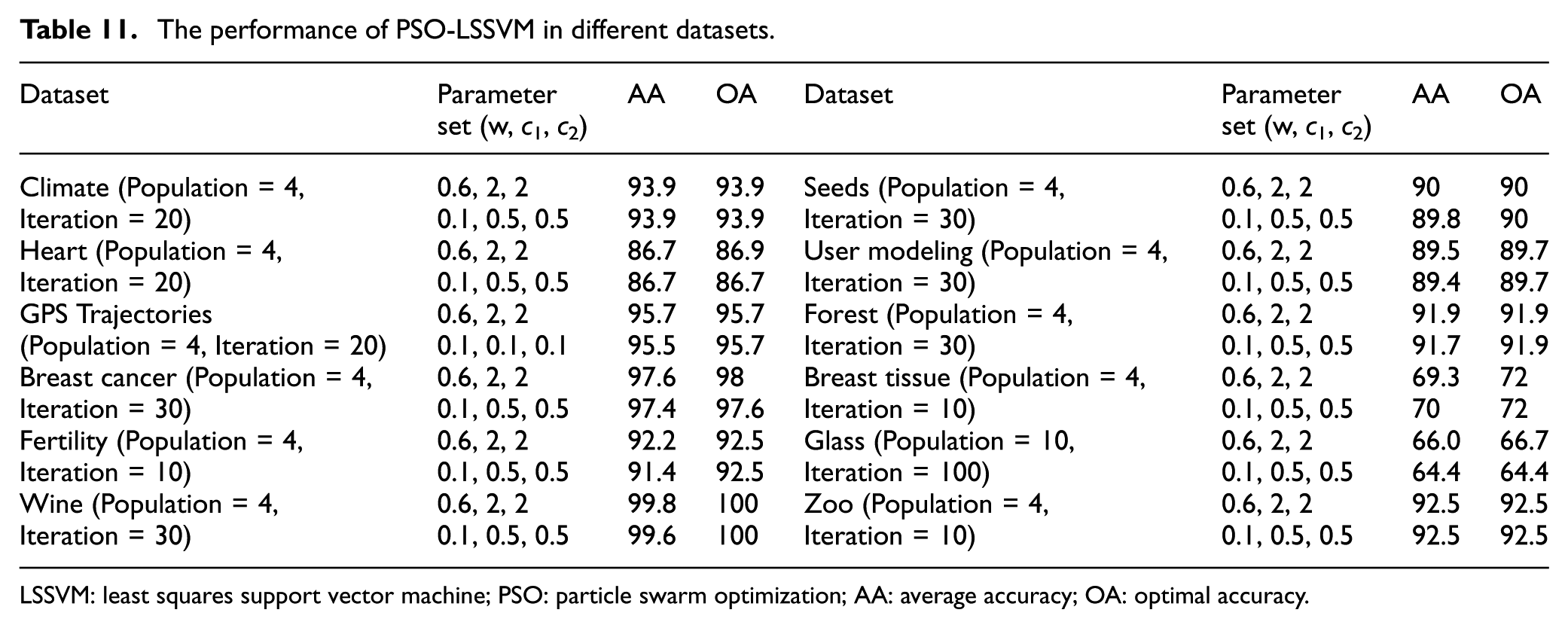
LSSVM: least squares support vector machine; PSO: particle swarm optimization; AA: average accuracy; OA: optimal accuracy.

Table 12.

The performance of ABC-LSSVM in different datasets.

Dataset	Parameter set (Limit)	AA	OA	Dataset	Parameter set (Limit)	AA	OA
Climate (Population = 4, Iteration = 30)	3	93.9	93.9	Seeds (Population = 4, Iteration = 30)	3	90	90
	10	93.9	93.9		10	90	90
Heart (Population = 4, Iteration = 50)	5	86.7	86.7	User modeling (Population = 4, Iteration = 30)	3	88.8	89.7
	20	86.7	86.7		10	88.5	89.7
GPS Trajectories (Population = 4, Iteration = 50)	5	95.7	95.7	Forest (Population = 4, Iteration = 50)	5	91.7	91.9
	20	95.5	95.7		20	91.8	91.9
Breast cancer (Population = 4, Iteration = 30)	3	97.6	98	Breast tissue (Population = 4, Iteration = 30)	3	70.4	72
	10	97.6	97.6		10	70.7	72
Fertility (Population = 4, Iteration = 30)	3	91.9	92.5	Glass (Population = 10, Iteration = 100)	5	64.4	64.4
	10	92.5	92.5		20	64.8	65.6
Wine (Population = 4, Iteration = 50)	5	99.1	100	Zoo (Population = 4, Iteration = 30)	5	92.5	92.5
	20	99.4	100		20	92.5	92.5

LSSVM: least squares support vector machine; ABC: artificial bee colony; AA: average accuracy; OA: optimal accuracy.

Table 13.

The performance of GA-LSSVM in different datasets.

Dataset	Parameter set (CP, MP)	AA	OA	Dataset	Parameter set (CP, MP)	AA	OA
Climate (Population = 4, Iteration = 10)	0.4, 0.01	93.6	93.9	Seeds (Population = 4, Iteration = 30)	0.4, 0.01	89.8	90
	0.8, 0.1	93.7	93.9		0.8, 0.1	89.8	90
Heart (Population = 4, Iteration = 10)	0.4, 0.01	86.2	86.7	User modeling (Population = 4, Iteration = 30)	0.4, 0.01	88.2	89.7
	0.8, 0.1	86.6	86.7		0.8, 0.1	87.1	89.7
GPS Trajectories (Population = 4, Iteration = 10)	0.4, 0.01	94.8	95.7	Forest (Population = 4, Iteration = 30)	0.4, 0.01	91.3	91.4
	0.8, 0.1	94.9	95.7		0.8, 0.1	91.5	91.9
Breast cancer (Population = 4, Iteration = 30)	0.4, 0.01	97.2	97.6	Breast tissue (Population = 4, Iteration = 10)	0.4, 0.01	67.1	68
	0.8, 0.1	97.3	97.6		0.8, 0.1	66.9	68
Fertility (Population = 4, Iteration = 10)	0.4, 0.01	90.6	92.5	Glass (Population = 10, Iteration = 100)	0.4, 0.01	64.4	64.4
	0.8, 0.1	91.1	92.5		0.8, 0.1	64.4	64.4
Wine (Population = 4, Iteration = 30)	0.4, 0.01	98.8	98.9	Zoo (Population = 4, Iteration = 10)	0.4, 0.01	92.5	92.5
	0.8, 0.1	99.3	100		0.8, 0.1	92.5	92.5

LSSVM: least squares support vector machine; GA: genetic algorithm; AA: average accuracy; OA: optimal accuracy; CP: crossover probability; MP: mutation probability.

As shown in Tables 11–13, PSO-LSSVM has the best performance in almost all the datasets with smaller iterations. ABC-LSSVM can also achieve a good accuracy with higher iterations. The performance of GA-LSSVM is acceptable with fast running speed. For binary classification tasks, SI-LSSVM has good performance (with an average accuracy around 90%). For multi-class classification tasks, SI-LSSVM also has good performance except “Breast Tissue” and “Glass” datasets. These two datasets have more categories but less attributes. This reveals that SI-LSSVM is not suitable for complex multi-class classification with lower attribute dimension. In binary classification and multi-class classification tasks with enough attributes, SI-LSSVM can achieve outstanding performance. PSO-LSSVM can obtain a better accuracy in shorter running time.

Comparative experiments with deep learning models on datasets with more samples and mixed features

We carried out more experiments on larger scale datasets with certain special features in this section. Details of these datasets are shown in Table 14. For “Gas sensor array under dynamic gas mixtures” dataset, stratified sampling method is used to select 80,000 instances.

Table 14.

Details of datasets (mixed features, larger).

Dataset	Class	Attributes	Sample feature	Attribute feature	Training set	Testing set
Heart 40	2	13	Multivariate	Categorical, Integer, Real	180	90
Wine 44	3	13	Multivariate	Integer, Real	124	54
Zoo 44	7	16	Multivariate	Categorical, Integer	70	31
Gas sensor array drift 48	6	128	Multivariate	Real	9737	4173
Gas sensor array drift (different concentrations) 48	6	128	Multivariate, Time-series	Real	9737	4173
Gas sensor array under dynamic gas mixtures 49	2	16	Multivariate, Time-series	Real	60,000	20,000

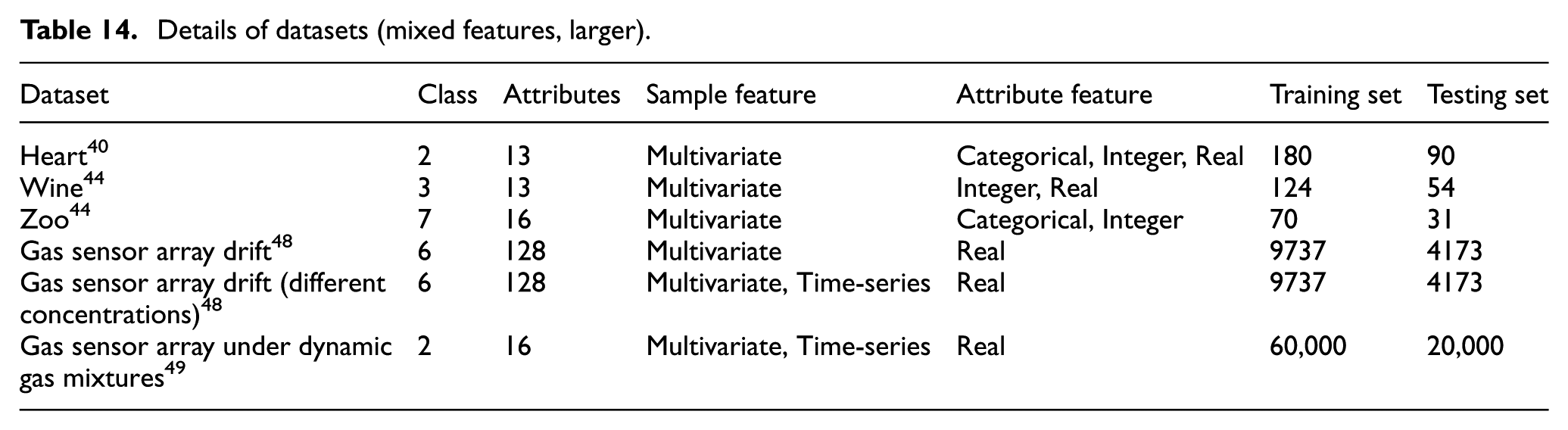
CNN and LSTM are selected as the comparisons. Considering the strong sequence analysis ability of LSTM, in experiments on time-series datasets like “Gas Sensor Array Drift (Different Concentrations)” dataset and “Gas sensor array under dynamic gas mixtures” dataset, every continuous five samples constitute a group with determined label. This strategy can help LSTM to exploit time information effectively.

In this section, all the experiments are conducted on a work station with Intel core(TM) i7-6700K CPU @ 4 GHz processor and 64 GB RAM. Software developing environment is Pycharm on 64 bit windows 7 system. For deep learning models, Keras with tensorflow backend is utilized as the development platform. CNN is built as a 9-layer structure: 2 convolution layers (64 convolution kernels with 1 × 3 size for Heart, Wine, Zoo and “Gas sensor array under dynamic gas mixtures” datasets; 512 convolution kernel with 1 × 3 size for “Gas Sensor Array Drift” and “Gas Sensor Array Drift (Different Concentrations)” datasets), 1 max-pooling layer, 2 convolution layers (128 convolution kernels with 1 × 3 size for Heart, Wine, Zoo and “Gas sensor array under dynamic gas mixtures” datasets; 1024 convolution kernel with 1 × 3 size for “Gas Sensor Array Drift” and “Gas Sensor Array Drift (Different Concentrations)” datasets), 1 global-average-pooling layer, dropout = 0.3, 2 dense layers (with 50 and 2 nodes respectively). relu function is selected as activation function, and binary cross entropy is selected as loss function. On time-series datasets, LSTM model with two LSTM layers and two dense layers are constructed. dropout = 0.25; sigmoid function is selected as activation function; binary cross entropy is selected as loss function. We use adaptive moment estimation optimizer. For large-scale datasets, batch_size = 20, nb_epoch = 200. In PSO, $w$ is set at 0.6, $c_1$  =  $c_1$  = 2. In ABC, limit is set at 20. In GA, crossover probability is set at 0.8 and mutation probability is set at 0.1. Binary coding strategy with 20 bits is used in our GA for each hyper parameter. Hyper parameters of LSSVM, γ and ${\sigma }^2$ , are selected among [0.01, 300].

As shown in Table 15, SI-LSSVM and deep learning models show different performance on datasets with different features:

1. On datasets with small samples such as Heart, Wine, and Zoo datasets, SI-LSSVM performs outstandingly;

2. For those datasets with different attribute features such as categorical or integer, PSO-LSSVM performs best;

3. CNN is very suitable for large-scale datasets. Along with the increase in sample size, the performance of CNN becomes better (Such as “Gas Sensor Array Drift” datasets); SI-LSSVM also has good performance on large-scale gas sensor data;

4. LSTM can obtain a better performance on “real” attribute and time series samples than CNN.

5. SI-LSSVM shows strong classification ability on relatively high-dimensional datasets such as Heart, Wine, Zoo, and Gas sensor datasets. On datasets with more categories and low dimension such as Glass datasets, SI-LSSVM has more room to be improved;

6. If the training set of LSTM becomes bigger, its performance will become better; on gas sensor datasets, when training set constitutes 60% of the dataset, average accuracy is 99.2%; when it constitutes 80%, average accuracy is 99.8%; this model can have a nearly 100% accuracy when it has 90% training set.

Table 15.

Experimental results compared with deep neural networks.

Dataset	Accuracy	PSO-LSSVM	ABC-LSSVM	GA-LSSVM	CNN	LSTM
Heart	AA	86.7	86.2	86.0	85.19	–
	OA	86.7	86.7	86.7	86.65	–
Wine	AA	99.8	99.4	99.2	99.3	–
	OA	100	100	100	100	–
Zoo	AA	98.77	98.25	96.93	98.39	–
	OA	100	100	99.06	100	–
Gas sensor array drift	AA	99.65	98.92	98.06	99.42	–
	OA	99.90	99.63	99.47	99.60	–
Gas sensor array drift (different concentrations)	AA	99.80	99.79	99.48	99.69	99.75
	OA	99.88	99.80	99.78	99.78	99.80
Gas sensor array under dynamic gas mixtures	AA	99.40	99.0	99.38	99.11	99.20
	OA	99.47	99.28	99.42	99.03	99.26

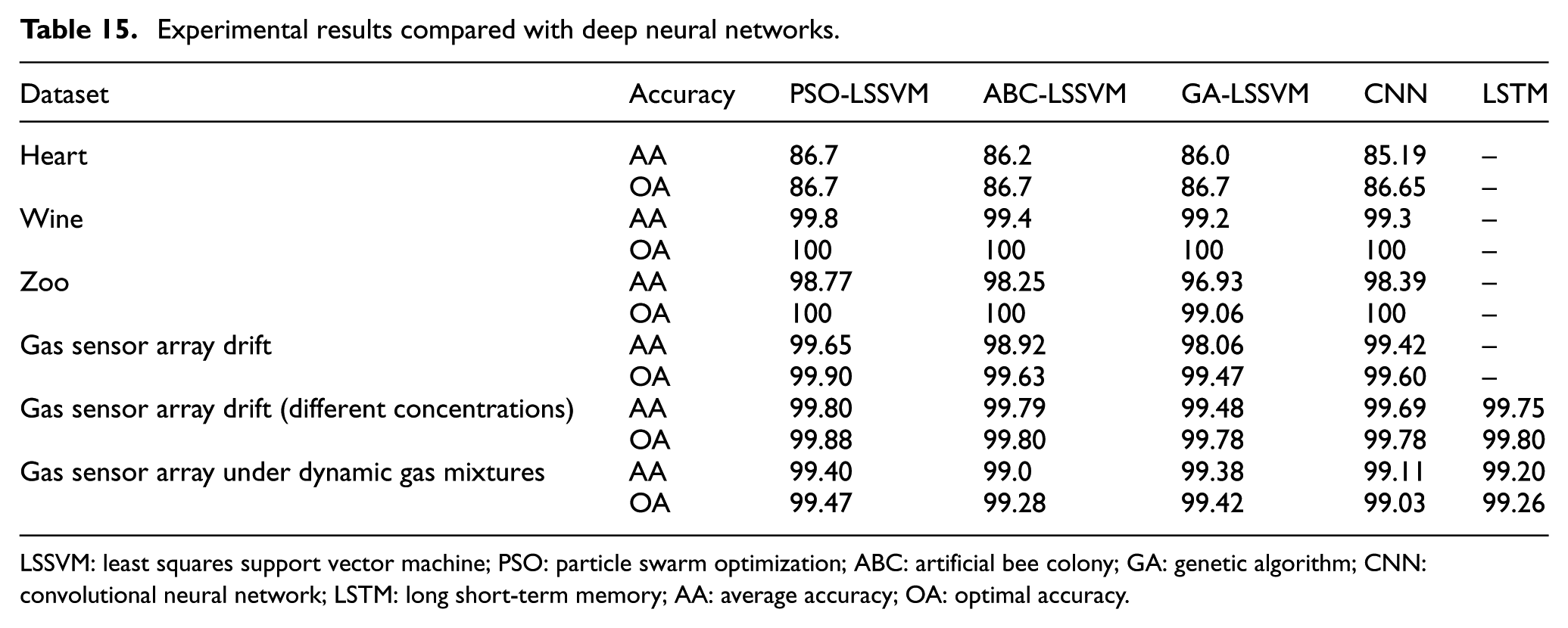
LSSVM: least squares support vector machine; PSO: particle swarm optimization; ABC: artificial bee colony; GA: genetic algorithm; CNN: convolutional neural network; LSTM: long short-term memory; AA: average accuracy; OA: optimal accuracy.

We hold the opinion that SI-LSSVM is more suitable than current deep neural networks in coal mine gas monitoring tasks due to the following reasons:

1. Deep learning is “data-thirsty.” Sometimes, deep neural networks need thousands of labeled samples in one task while the negative samples about coal mine safety situation, mine disasters, must be small and limited;

2. We always need fast response speed in this scenario but the computation time of deep neural networks is relative long;

3. Deep learning models have good performance in perceptual tasks especially good at numeric and continuous data such as speeches and images. In our data as Table 17 in this article, there is a nominal attribute, “damage type.” For data like this, SI-LSSVM is more effective.

Computational time complexity analysis of SI-LSSVM

In SVM, since the algorithm needs to handle the quadratic convex optimization, the computational time complexity is $\mathrm{O}(n^3)$ . Here, n is the dimension of input samples. In LSSVM, the inequality is replaced by equation and the quadratic programming is changed into a liner problem. Therefore, the complexity is reduced to $\mathrm{O}(n^2)$ .^50,51

For swarm intelligence algorithms, the time complexity is closely correlated with the problem to be optimized. In SI-LSSVM, {γ, ${\sigma }^2$ }, two parameters are optimized by PSO, ABC, and GA. The dimension of each individual is 2 and it is unrelated to n.

In PSO, the main program statement in the loop is the speed updating formula for particles. In this formula, 5 multiplication operations and 5 addition operations are needed. For a PSO with n particles and m iterations, the computational time can be written as equation (22)

$$T_{\mathrm{PSO}-\mathrm{LSSVM}}=m\times n\times (2\times T_{\mathrm{update}}+T_{\mathrm{LSSVM}}+T_{\mathrm{best}})$$

(22)

where $T_{\mathrm{LSSVM}}$ is the time for evaluating the particle, also the time for LSSVM classification; $T_{\mathrm{best}}$ is time for the updating process of pbest, gbest with a O(n) complexity. Then, the computational time complexity of PSO-LSSVM can be considered as $\mathrm{O}(n^4)$ .

The computation time of ABC-LSSVM can be illustrated as equation (23)

$$T_{\mathrm{ABC}-\mathrm{LSSVM}}=m\times (2(a\times T_{\mathrm{employed}}+b\times T_{\mathrm{onlooker}}+c\times T_{\mathrm{scouts}})+n\times T_{\mathrm{LSSVM}})$$

(23)

where $T_{\mathrm{employed}}$ , $T_{\mathrm{onlooker}}$ , $T_{\mathrm{scouts}}$ , and $T_{\mathrm{LSSVM}}$ are the time for employed bees, onlooker bees, scouts, and LSSVM; a + b + c = n. The complexity of $T_{\mathrm{onlooker}}$ is $\mathrm{O}(n)$ . (In selection operation, n probability need to be calculated). Due to the fact that the computational complexity of LSSVM is $\mathrm{O}(n^2)$ , the complexity of ABC-LSSVM is $\mathrm{O}(n^4)$ .

In GA-LSSVM, similarly, the time can be approximately represented as equation (24). The complexity of selection, crossover, and mutation operations is regarded as $\mathrm{O}(n)$ , $\mathrm{O}(1)$ , $\mathrm{O}(1)$

$$T_{\mathrm{GA}-\mathrm{LSSVM}}=m\times n\times (2T_s+2T_c+2T_m+T_{\mathrm{LSSVM}})$$

(24)

where $T_s$ , $T_c$ , $T_m$ , and $T_{\mathrm{LSSVM}}$ are the time for selection, crossover, mutation operations, and LSSVM. Computational time complexity of this algorithm can also be regarded as $\mathrm{O}(n^4)$ .

Thus, we can conclude that computational time complexity of SI-LSSVM is $\mathrm{O}(n^4)$ .

Gas monitoring based on SI-LSSVM

The description of coal mine data

In this article, SI-LSSVM models are applied to evaluate the safety status of two real coal mines in china. Statistical features of these two datasets, “obvious risk assessment” dataset ⁵² and “coal mine gas and environment” dataset, ⁵³ are shown in Table 16. Detailed samples are listed in Tables 17 and 18, respectively.

Table 16.

Statistical features of two real coal mine datasets.

Dataset	Class	Attributes	Training set	Testing set
Obvious risk assessment	2	5	12	6
Gas and environment	5	6	10	10

Table 17.

Samples of obvious risk assessment dataset.

Number	Gas pressure (MPa)	Ruggedness coefficient (f)	Initial gas diffusion speed (m/s)	Damage type	Mining depth (m)	Obvious risk
1	2.11	0.32	16.50	3	739	Yes
2	2.10	0.43	10.30	3	539	Yes
3	0.78	0.54	5.50	1	535	No
4	2.63	0.34	13.00	5	547	Yes
5	1.93	0.59	6.30	1	499	No
6	1.99	0.39	11.10	3	495	Yes
7	0.69	0.51	4.50	2	516	No
8	2.77	0.31	12.00	5	545	Yes
9	1.34	0.28	10.60	2	489	Yes
10	2.01	0.39	9.90	4	589	Yes
11	0.71	0.46	5.70	2	445	No
12	2.00	0.52	14.60	3	870	Yes
13	2.84	0.45	13.10	3	456	Yes
14	0.85	0.49	5.80	1	542	No
15	1.83	0.30	9.30	3	503	Yes
16	2.39	0.37	10.10	3	698	Yes
17	0.78	0.37	6.50	2	526	No
18	2.57	0.52	11.60	3	845	Yes

Table 18.

Samples of coal mine gas and environment dataset.

Number	H2S (%)	Temperature (°C)	Wind speed (m/s)	CH4 (%)	CO (%)	O2 (%)	Safety status
1	0.00410	26.5	1.14	0.90	0.00230	18.7	4
2	0.00065	21.5	1.87	0.25	0.00018	19.3	1
3	0.00066	23.8	2.48	0.57	0.00085	19.6	2
4	0.00071	25.9	1.98	0.65	0.00140	18.2	3
11	0.00062	30.7	0.56	1.01	0.00240	20.7	5
5	0.00107	18.0	0.81	0.31	0.00045	20.1	1
6	0.00085	27.4	1.35	0.89	0.00195	19.3	4
7	0.00050	23.1	2.01	0.45	0.00070	20.6	2
8	0.00092	24.3	1.55	0.70	0.00130	19.4	3
9	0.00042	22.2	2.21	0.53	0.00090	20.3	2
10	0.00074	27.9	1.48	0.82	0.00190	18.9	4
12	0.00052	22.0	2.56	0.36	0.00050	19.5	1
13	0.00041	25.2	1.63	0.73	0.00160	19.2	3
14	0.00052	26.1	1.50	0.85	0.00200	20.5	4
15	0.00070	22.7	2.32	0.49	0.00080	19.4	2
16	0.00065	19.5	3.35	0.19	0.00020	18.8	1
17	0.00419	24.0	1.75	0.71	0.00150	20.7	3
18	0.00229	28.9	0.89	1.05	0.00250	18.1	5
19	0.00069	29.6	0.96	1.08	0.00245	19.5	5
20	0.00071	28.5	0.48	1.03	0.00251	18.3	5

Experiments and analyses

In order to prevent mine disasters, SI-LSSVM models are utilized to monitor safety status of these two mines. We use the similar experimental setting as written in section “Detailed comparative experiments.” The performances of SI-LSSVM on obvious risk assessment dataset can be illustrated in Table 19 and Figure 5.

Table 19.

Experimental results of SI-LSSVM on obvious risk assessment dataset.

Obvious risk assessment dataset	Population	Iteration	Accuracy	$\mathbf{\gamma }$	${\mathbf{\sigma }}^2$	Training time	Testing time
PSO-LSSVM	4	50	100	92.7513	18.1128	3.1	1.63
	4	25	100	61.4771	82.264	1.6	1.55
	4	25	100	31.5341	173.592	1.6	1.66
ABC-LSSVM	4	50	100	260.047	225.022	3.4	1.55
	4	25	100	131.391	92.394	2.1	1.52
	4	25	100	229.124	284.592	2.2	1.55
GA-LSSVM	4	50	100	102.932	180.536	3.1	1.52
	4	25	100	67.4318	187.978	1.7	1.54
	4	25	100	57.2483	130.165	1.6	1.48
Cross-validation	–	–	100	1.7082	2.1385	3.3	1.62
	–	–	100	1.7284	2.6101	3.3	1.51
	–	–	100	1.4887	2.6453	3.3	1.58
Default parameters	–	–	100	10	10	1.6	1.52
	–	–	83.3	10	0.2	1.5	1.61

SI: swarm intelligence; LSSVM: least squares support vector machine; PSO: particle swarm optimization; ABC: artificial bee colony; GA: genetic algorithm.

Figure 5.

Fitness curves of three algorithms on obvious risk assessment dataset.

As listed in Table 10, apart from man-made strategy, almost all the models perform outstandingly in obvious risk assessment dataset. This is probably because those features for risk assessment are more distinct and notable. All the SI-LSSVM models can obtain the best parameters and classify samples correctly in a short time, as shown in Figure 5.

On “coal mine gas and environment” dataset, as illustrated in Table 20 and Figure 6, SI-LSSVM also performs better than other optimization methods. Among those models, PSO is the best optimizer which can easily gain the suitable parameters for LSSVM. ABC-LSSVM also has an outstanding performance although its average accuracy is a little lower than PSO-LSSVM. GA-LSSVM can get an acceptable classification accuracy with the shortest training time.

Table 20.

Experimental results of algorithms on coal mine gas and environment dataset.

Coal mine gas and environment	Population	Iteration	Accuracy	$\mathbf{\gamma }$	${\mathbf{\sigma }}^2$	Training time	Testing time
PSO-LSSVM	20	200	90	9.56945	3.13043	173.2	0.45
	10	200	90	155.679	2.34177	88	0.49
	10	100	90	300	2.05442	46.9	0.43
	6	100	80	185.4234	1.0650	29.1	0.45
	6	100	90	9.90224	3.28786	25.1	0.49
	4	50	90	11.0396	2.2851	9.3	0.48
	4	50	90	14.6609	2.36429	9.6	0.56
	4	50	90	203.357	1.98496	10.1	0.51
	4	50	80	4.77531	1.30197	9.9	0.44
	4	50	80	1.01627	3.952	9.7	0.47
Average accuracy and time (9 times)	4	50	87.5	–	–	9.5	0.47
	6	100	88.75	–	–	26.6	0.48
ABC-LSSVM	20	200	90	256.659	2.12783	185.8	0.46
	10	200	90	29.7115	2.70611	85.5	0.52
	10	100	90	218.939	2.13241	45.2	0.54
	6	100	80	70.4943	8.2118	27.4	0.40
	6	100	90	2.76284	22.3091	29.5	0.55
	4	50	80	275.3262	0.9475	11.6	0.52
	4	50	90	11.1828	2.43557	12.2	0.55
	4	50	90	201.815	2.37844	11.5	0.42
	4	50	90	71.2999	2.08036	11.6	0.51
	4	50	90	19.9078	3.19623	12.7	0.41
Average accuracy and time (9 times)	4	50	86.25	–	–	11.9	0.44
	6	100	87.5	–	–	28.8	0.42
GA-LSSVM	20	200	90	19.9853	57.6663	137.4	0.52
	10	200	90	201.398	2.07187	83.6	0.50
	10	100	90	54.6265	2.95418	43.5	0.41
	6	100	70	167.435	64.2619	24.7	0.52
	6	100	90	240.679	2.74391	23.8	0.44
	4	50	70	253.917	65.6478	11.5	0.53
	4	50	70	23.0339	7.8192	11.4	0.49
	4	50	70	243.557	83.9385	10.8	0.51
	4	50	80	118.144	1.34834	12.1	0.43
	4	50	90	212.041	2.50445	11.4	0.55
Average accuracy and time (9 times)	4	50	75	–	–	12.0	0.49
	6	100	78.75	–	–	24.2	0.47
Cross-validation	–	–	80	1.4107	1.4405	8.7	0.35
	–	–	80	2.1816	1.3152	7.9	0.44
	–	–	80	2.5325	1.2602	7.4	0.35
Default parameters	–	–	70	10	10	0.4	0.42
	–	–	70	10	0.2	0.3	0.31

LSSVM: least squares support vector machine; PSO: particle swarm optimization; ABC: artificial bee colony; GA: genetic algorithm.

Figure 6.

Fitness curves of three algorithms on coal mine gas and environment dataset (best fitness in the median run of 9 runs).

The testing time is around 0.5 s, which illustrates that those models can monitor gas status timely.

Conclusion

In this article, we studied LSSVM optimized by three major swarm intelligence techniques: PSO, ABC, and GA. A number of comparative experiments and analyses are conducted on public testing dataset. Experimental results show that swarm intelligence techniques can effectively select the hyper parameters for LSSVM. This SI-LSSVM model can sort samples both from UCI datasets and real coal mine datasets fast and accurately, thereby can prevent coal mine disasters validly. In our experiments, these optimization methods perform differently in different datasets:

1. PSO is the best optimizer which can obtain better parameters with smaller swarm size and shorter time.

2. ABC also performs outstanding with a longer training time.

3. GA has a better performance than cross-validation and default parameters; the training time of GA is shortest.

SI-LSSVM has several special features compared with deep learning models:

1. This model can effectively deal with those datasets with smaller samples and categorical attributes.

2. On the datasets with more categories and lower dimension, SI-LSSVM has room to be improved.

We hope to make more improvements in our future work and introduce deep models appropriately:

1. Suitable training strategies and improved deep models are expected so as to deal with those datasets with small samples appropriately. A feasible solution is the application of transfer learning techniques.

2. The results of deep neural networks can be used as the inputs of SI-LSSVM. For example, we can determine the damage type by the use of CNN to perceive the visual information of coal mine workplace; we can also predict the concentration of certain gas in future by the use of RNN to deal with time-series arisen from gas sensors. These outputs can constitute the input vector of SI-LSSVM and help the algorithm fulfill gas monitoring task.

3. This model can also be developed by other data processing strategies such as principal component analysis (PCA) ⁵⁴ or SI-based feature selection, ⁵⁵ entropy-based evaluation, ⁵⁶ and hybrid SI algorithms ⁵⁷ so as to handle more complex coal mine gas sensor data.

Overall, as the classical statistical learning strategy, LSSVM can be widely applied in risk assessment tasks in mining workplace.