Sage Journals: Discover world-class research

Abstract

Although much work has been done since wireless sensor networks appeared, there is not a great deal of information available on real deployments that incorporate basic features associated with these networks, in particular multihop routing and long lifetimes features. In this article, an environmental monitoring application (Internet of Things oriented) is described, where temperature and relative humidity samples are taken by each mote at a rate of 2 samples/min and sent to a sink using multihop routing. Our goal is to analyse the different strategies to gather the information from the different motes in this context. The trade-offs between ‘sending always’ and ‘buffering locally’ approaches were analysed and validated experimentally, taking into account power consumption, lifetime, efficiency and reliability. When buffering locally, different options were considered such as saving in either local RAM or FLASH memory, as well different alternatives to reduce overhead with different packet sizes. The conclusion is that in terms of energy and durability, the best option is to reduce the overhead. Nevertheless, sending larger packets is not worthy when the probability of retransmission is high. If real-time monitoring is required, then sending always is better than buffering locally.

Keywords

Wireless sensor network environmental monitoring TinyOS real deployment Internet of Things communication strategies

Introduction

Internet of Things (IoT) platforms are the basis for new value systems and the guide for development of new applications. However, all these things require the coordination of several elements: IoT platforms, efficient and wide-range communications, robust control, simple and reliable management and security. In combination with wireless sensor networks, IoT systems become a powerful tool to sense the environment, although some requirements are necessary for specific data gathering, like audio or video.¹

A wireless sensor network (WSN) is a set of nodes, also called motes, which have wireless communication and processing capabilities. These nodes work in a collaborative way, implementing multihop routing protocols designed to aid the collection of data gathered by sensors on all nodes by a data sink. WSN is useful in monitoring applications where the nodes collect data about one or more parameters over a large area. Motes are low-power, low-performance devices, equipped with a microcontroller system with a CPU and memories (RAM and FLASH), a radio frequency chipset following the IEEE 802.15.4:2006 standard,² various sensors and an autonomous power supply (in most cases, two AA batteries). In general, this technology has been consolidated and several hardware and software options are currently available. One of the most widely used hardware and software systems is TelosB motes,^3,4 with the TinyOS operating system,^5,6 designed specifically for use in motes. There are several combinations for hardware and software as shown in Strazdins et al.;⁷ nevertheless, as shown in Delamo et al.,⁸ this combination (TelosB and TinyOS) is still the most optimum in terms of reliability, network lifetime and efficiency.

WSN has many applications, but lend themselves particularly well to environmental monitoring (EM).^9,10 On one hand, applications such as Harvester¹¹ based on TinyOS (discussed in more detail in section ‘Hardware and software: TelosB and TinyOS’) allow the installation of many sensors over a large area, without the need for any form of network infrastructure, making the collection of accurate data from a large area an easy task. On the other hand, most commercially available motes include temperature (T), relative humidity (RH) and light sensors as standard, and it is easy to add other external sensors to augment the number of parameters to be monitored.

In the application to be discussed here, data for meteorological studies (T and RH) must consist of a series of readings taken at 10-min intervals. Each reading is the average of a series of samples taken every 30 s during the 10- and 50-min period in question. The sampling frequency is determined by the accuracy of the sensors used and the margin of error we wish to assume. The formula used for the estimation of the different meteorological variables can be found in environmental protection agency (EPA).¹² Following this criteria, we determine that for our sensors, as described in section ‘Design issues for EM applications’, a sampling period of 30 s is sufficient to provide accurate results. Further information and a complete guide to develop similar applications can be found in Delamo et al.⁸

In the design of these EM applications, different options are available for processing the data and calculating the 10-min averages. There is a trade-off between two different approaches, ‘sending always’ versus ‘buffering locally’. This is our goal. The former option avoids saving data locally and improves real-time performance, but requires transmitting many packets. The latter option reduces the number of data packets sent and allows local processing of the 10-min average, but requires data to be saved locally in the motes. In the case of local buffering of the data, we will evaluate two different implementations, the first sends each 10-min average in a single packet and the second fits as many 10-min averages as possible in a single packet without fragmentation, maximizing the payload and reducing the overhead. Thus, the contribution of this article is to study and analyse experimentally the advantages and disadvantages of both the ‘send always’ and ‘buffering locally’ strategies.

The rest of the paper is structured as follows. In section ‘Related works’, we analyse the related work. In section ‘Hardware and software: TelosB and TinyOS’, we briefly introduce the hardware and software elements of the network: TelosB motes and the TinyOS operating system. In section ‘Design issues for EM applications’, we look at the design issues that must be taken into account when designing an application for EM. In section ‘Send always versus buffering locally’, we analyse the behaviour and results over a real deployment of the two different approaches, send always and buffering locally, before concluding with a discussion and analysis of the results in section ‘Analysis and evaluation of send always and buffering locally approaches under a real WSN deployment’.

Related works

WSNs have been used in many different applications, such as EM, precision agriculture, habitat monitoring, with real deployments, most of them were analysed in Strazdins et al.⁷ Some of these deployments are worth mentioning. Dozer¹³ shows an ultra-low-power data gathering application, based on TinyOS, using TDMA MAC (Time Division Multiple Access Media Access Control) and multihop routing. Dozer achieves an average duty cycle of less than 0.2%, using a sampling period of 2 min. SensorScope¹⁴ explains the difficulties in EM in harsh conditions, using TinyOS, with a global synchronized duty-cycle MAC algorithm as well as multihop routing. GreenOrbs is a large-scale WSN for forest monitoring and research, used to carry out performance analysis and scalability properties.¹⁵ The software part of sensor scope is based on TinyOS and Collection Tree Protocol (CTP)¹⁶ routing protocol using TelosB motes. Finally, in Gallart et al.,¹⁷ it is described the deployment of a low-cost WSN for EM in an urban street, also based on TelosB motes running TinyOS.

In addition, in the literature, we find relevant works that help us to improve the performance of WSN. In Aguirre-Guerrero et al.,¹⁸ the authors consider different strategies for distributed congestion control in WSN for a fair packet delivery between nodes, while at the same time, the network congestion is mitigated using adaptive traffic mechanisms. In Yang et al.,¹⁹ we find different optimization techniques for node deployment in real scenarios, in particular at oilfields, where the major concern is the optimum placement of nodes to ensure the full connectivity. Finally, in Gana Kolo et al.,²⁰ the authors show an adaptive lightweight lossless data compression mechanism to improve network efficiency.

Finally, we can find previous studies related to the topic of this article, both in the design aspects of the EM application itself and in the analysis of the trade-off between the send always and buffering locally approaches. In Zennaro et al.,²¹ the authors study the temporal and energy characteristics of a 2.4 GHz sensor network in an outdoor environment. They suggest that when deploying WSN in real world scenarios, the sampling periods of sensor networks should be adjusted according to distance to normalize battery lifetime as well as running more accurate energy-aware routing protocols. From another point of view, Mathur et al.²² studied on detail the power consumption of various processes, including the transmission of data over the radio and saving data to various storage devices.

Although all these papers help to find out the basic features associated with WSN such as multihop routing and long lifetimes over real deployments, WSN is a non-trivial task and many issues remain still open. Due to the complexity and low-performance on the devices on these networks, very few real deployments are found.⁷ The weak point of these networks is the wireless communication because it is difficult to implement an efficient and reliable data transmission. Thus, in this article, we evaluated experimentally the trade-offs between several strategies to perform this task.

Hardware and software: TelosB and TinyOS

In this section, we will introduce the mote hardware and software, focusing on one of the most widely used combinations; TelosB motes with the TinyOS operating system.

TelosB mote

TelosB mote is an ultra-low-power wireless device, suitable for use in sensor networks and monitoring applications. The TelosB hardware includes a Texas Instruments 8 MHz MSP430 F1611 microcontroller, a 32 kHz oscillator, a Chipcon CC2420 2.4 GHz IEEE 802.15.4:2006 compliant radio,² 10 kB of on-chip RAM, 48 kB on-chip flash, a further 1 MB of on-board flash memory (STM25P80 from STMicroelectronics), an integrated Planar Inverted Folded Antenna (PIFA) and an SubMiniature version A (SMA) coax connection for an external antenna. It is important to highlight that the CC2420 transceiver allows the detection of start frame delimiter (SFD) in IEEE 802.15.4 frames that will help to improve time accuracy.²³ In addition, TelosB motes embedded high-quality sensors to measure T and RH. Since these motes are not suitable for transmission over long distances, we require the collaboration of the different motes to create a path to the sink using multihop routing.

Finally, it must be noted that this mote may show some drawbacks such as the lack of a radio frequency (RF) amplifier or it only works in the 2.4 GHz band. However, these weaknesses can be overcome using TelosB compatible commercial motes with RF amplifiers that can be found in the market or using external antennas with higher gain.⁸

TinyOS

TinyOS^5,6 is an open-source operating system designed for low-power wireless devices. TinyOS supports multiple microcontroller families and radio chips. It includes a large repository of components that can be combined for fast prototyping of new applications. TinyOS has become one of the most used operating systems for WSN applications due to its performance, good adaptation to WSN requirements and widespread acceptation by researchers and company developers.

Several tools suitable for EM applications are available in the repository.⁵ To the best of our knowledge, only two complete EM applications capable of data gathering with multihop routing and low-power listening operation at the MAC layer are freely available The first application is “Boomerang”, a pioneering application developed by the Moteiv Company, which was integrated in a specific TinyOS distribution. This application includes a synchronous low-power listening (LPL) MAC protocol,²⁴ periodically flooding the entire network with broadcast packets containing its local time. The routing protocol used in Boomerang is the well-known MultihopLQI, which establishes a routing tree from every node to the sink using the link quality LQI as the routing metric. The second application is Harvester,¹¹ a low-power, open-source, data gathering application developed by researchers from the Computer Engineering and Networks Laboratory of the ETH, Zurich. In this work, the Harvester tool has been implemented. This tool will be explained in detail in the next sections. Finally, it is worth mentioning that there are other interesting operating systems for these motes, such as Contiki, but it is less efficient in terms of energy when compared with TinyOS.⁸

Design issues for EM applications

Several issues must be taken into account when designing a WSN application for EM.⁸ The first of these is the need to reduce energy consumption as much as possible to improve the lifetime of the network. Second, the reliability of the motes and the data collection must be maintained or improved. Finally, the accuracy of the measurements taken by the sensors must be within the desired levels.

As it has been mentioned, Harvester¹¹ is a low-power, open-source data gathering application developed by researchers from the Computer Engineering and Networks Laboratory of the ETH, Zurich, which is freely available in the TinyOS repository. It is composed of two layers: the application layer, which performs the sensor sampling, topology discovery and data status analysing of the nodes, and the protocol stack, composed of a synchronization stack at the MAC level, and modifications to the CTP protocol,¹⁶ using LPL.²⁴ For the enhancements in Harvester to be implemented, modifications to LPL have been made. These include changing the power cycling of the radio to a predictable wake-up schedule, adding time information in the packets sent and adding wake-up prediction for neighbouring nodes.

Since one of the most critical areas in WSN design is that of power consumption, several methods are used in Harvester in order to reduce it as much as possible. At the MAC level, there is a modified version of the typical TinyOS low-power listening (LPL) protocol that is capable to estimate the duty cycle of the neighbouring nodes. It must be noted that TelosB motes allows high temporal accuracy for the MAC time stamping using SFD pin by CC2420 transceiver. Using this information, a node can start its transmissions according to the estimated wake-up schedule of the intended receiver. The routing layer in Harvester is based on the CTP that builds a routing tree to collect the data in one or several network sinks, based on multihop behaviour. CTP is a best-effort routing protocol that makes use of expected transmission (ETX) as the routing metric to determine the best path to one sink. The protocol is not completely reliable, since each packet is sent from its source only once. It is then ‘collected’ by the protocol and forwarded to the sink. The sink cannot notice that a packet has been sent, so cannot request a resend if it does not arrive. Similarly, no acknowledgement is sent by the sink when it receives a packet, so the source has no way of determining whether the packet has arrived correctly.

While Harvester shows increased power savings over the standard MAC protocol, it works on a ‘send always’ philosophy sending every 30 s by default. E-Harvester (Enhanced Harvester) is a modified version of Harvester that in addition, it includes a ‘buffering locally’ approach to reduce the number of packets to be sent while increasing the reliability of the transmissions by sending all packets twice. Developed at the Department of Computer Science, University of Valencia, details of the application can be found in Delamo et al.⁸ and Gallart et al.¹⁷ Thus, E-Harvester we can run in the motes both strategies ‘send always’ and ‘buffering locally’. This tool will be used in order to analyse both approaches. In addition, we can configure the ‘buffering locally’ approach to send packets with different payloads, to send the information gathered at each motes from different time periods. It must be stressed that we can find other routing protocols such as Routing Protocol for Low-Power and Lossy Networks (RPL) to deliver the information to the sink, but according to Ogawa et al.²⁵ after a thorough analysis on TelosB motes, the authors conclude that CTP is more reliable than RPL, because the loss rate is smaller, it needs less memory and is more efficient in terms of energy.

Send always versus buffering locally

When E-Harvester is running a ‘send always’ approach, it will transmit a packet for each reading taken from the sensors. When a node sensor is triggered, taking a sample from each of the sensors, they are immediately encapsulated in a packet and sent via the radio component to the father node. While in some situations this immediate sending of packets may be beneficial, it causes a high number of small packets to be sent, which may not provide the most efficient use of the radio. This strategy is useful in real-time monitoring, but in many cases, data are not analysed in real time and there is no need to send all data immediately.

Since the radio component of the mote has a high-power requirement (see Table 1), it should be used as little as possible in order to reduce the total power consumption of the mote.²² If there is no need to send each sensor reading immediately, we can reduce the use of the radio by saving each reading locally and sending them together in a single packet. This can be configured in E-Harvester too using the ‘buffering locally’ approach.

Table 1.

Comparison of energy cost for communication and storage processes in a TelosB mote.

Hardware	Description	Process	Energy ( $μ J$ )
CC2420	Radio chipset	Sending 1 byte	1.5
STM25P80	External flash memory	Adding 1 byte write and read cycles	0.368
MSP430 instruction	Microcontroller instruction	Touching a byte in RAM	0.0008

In addition, there are two possible solutions for local buffering of data in the motes: local RAM and FLASH memory. Since all data provided by the sensors must be stored in RAM before being transmitted, no extra cost is incurred if it is stored but not transmitted immediately. Storing the data in the FLASH memory is possible, but the energy cost is much higher than storing in RAM, as can be seen in Table 1. The FLASH memory requires a minimum of 2.7 V, which makes its long-term use in a mote unfeasible. Also, since the data for each 10-min period occupy very little space, the RAM has enough capacity to hold all the data that can be sent in a single packet.

We will now analyse the packets sent by the radio in each approach and their energy cost. The packets sent by the ‘send always’ approach include a fixed overhead of 26 bytes in all cases, of which 11 bytes correspond to the packet header and 15 bytes are a fixed overhead required by the CTP and included in the packet payload. The payload of each packet varies, depending on the amount of data to be sent. In this approach, the payload is 24 bytes: 15 bytes for the CTP and 9 bytes for the actual data. Table 2 shows the various fields within the payload and the bytes assigned to each one.

Table 2.

Packet payload when using the send always and buffering locally (10 and 50 min) approach.

Field description	Send always (bytes)	Buffering locally for 10 min (bytes)	Buffering locally for 50 min (bytes)
CTP	15	15	15
Mote ID	2	2	2
Sequence Number	1	1	1
Temperature	2	4	20
Relative humidity	2	4	20
Number of OK measurements	−	1	5
Control	−	1	1
Internal voltage (battery level)	−	2	2
Total payload	24	30	66

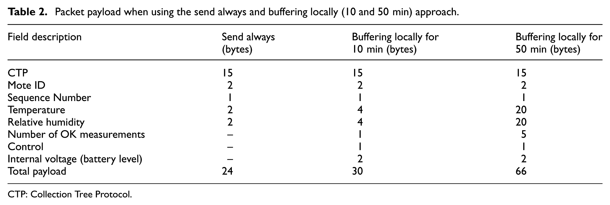
CTP: Collection Tree Protocol.

In the ‘buffering locally’ approach for 10-min period, the sensors continue to provide readings at 30-s intervals, but the total value of all the readings is calculated by the mote and saved in the RAM. If a reading is deemed to be an error or invalid (due to an unusually high or low value), it is ignored. Once 20 readings have been taken and the total value has been calculated, ignoring any invalid reading, the total value for the sum of all correct readings is sent to the sink, along with the number of correct readings taken (in order to accurately calculate the average). Since the total value for the sum of all readings is substantially higher than the value of just one reading, the fields for temperature and humidity have been increased in size to 4 bytes each. The other payload fields (mote ID, sequence number and battery voltage level) remain the same, but two new fields of 1 byte each are added for control. The third column in Table 2 shows the content of the payload when the ‘buffering locally’ approach for 10-min period approach is used. The total payload is 30 bytes with ‘buffering locally’ approach only 6 bytes more than in the ‘send always’ approach. The main difference between the two approaches is that for any 10-min period, ‘send always’ sends 20 packets, while ‘buffering locally’ for 10-min period only sends 1 packet, resulting in much less packet overhead with the latter. Regardless of the payload size, packet overhead remains the same; further reductions in overhead can be made by maximizing the payload of each packet in the buffering locally approach.

However, as we mentioned above, the payload size of each packet is variable and we could fit E-Harvester in order to carry more information. In this case, TinyOS must reserve sufficient space in the RAM for the largest possible packet. This is done by modifying the variable TOSH_DATA_LENGTH in TinyOS. Although larger payloads are possible in some configurations, we have found that if TOSH_DATA_LENGTH is set to more than 69 bytes, the programming of the motes does not compile correctly. Increasing the payload size also increases the demands on the RAM of all motes, as all packets are increased in size, requiring more RAM for queuing the packets.

When setting TOSH_DATA_LENGTH (the maximum payload size) to 69 bytes, a total of 54 bytes are available for the actual data because 15 bytes are required by the CTP. Since all data are from the same mote, the mote ID, sequence number, there is no need to duplicate control byte and battery voltage fields. Every 10-min period added to the packet requires only 9 extra bytes, 4 bytes for the temperature, 4 bytes for the humidity and 1 byte for the number of correct readings. Taking into account the maximum of 69 bytes and the fields whose size does not vary (CTP, mote ID, sequence number, control and voltage), 21 bytes in total, we can calculate the number of 10-min periods that can be included in a single packet

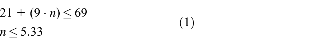
\begin{matrix} 21 + (9 \cdot n) \leq 69 \\ n \leq 5.33 \end{matrix}

(1)

where fixed fields are the CTP, mote ID, sequence number, control and voltage fields whose value does not change and n is the number of 10-min periods. The maximum possible value for n is 5, which results in a total payload size of 66 bytes, as seen in the fourth column in Table 2. This configuration is called ‘buffering locally’ approach for 50-min period.

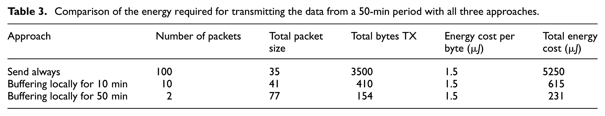
Once we have analysed the payload and overhead for each approach, we can compare the energy requirements of each of them. In the first approach, the total number of bytes transmitted by the radio for each packet is 35 (11 bytes for the header and 24 bytes payload). When saving the data locally and sending packets at 10-min intervals, 41 bytes are transmitted by the radio. Finally, when saving the data from five 10-min periods and maximizing the packet size, a single packet of 77 bytes is sent every 50 min. Note as explained in section ‘Design issues for EM applications’ that in the two buffering locally approaches, each packet is sent twice. This is a deliberate measure, designed to improve the reliability of the data collection.

In order to easily compare the energy cost of each approach, we will compare them for a sample collection period of 50 min. The results can be seen in Table 3, where it is clear that the two buffering locally approaches require much less energy to transmit the same number of sensor readings to the sink. It must be noted that this information only is available taking into account the data exchanged by the application itself. This means that, we have not included the detail of routing, synchronization protocols or even MAC overhead because they are related to the network conditions (environment) and they will vary due to the dynamic features of these WSN and their channels.

Table 3.

Comparison of the energy required for transmitting the data from a 50-min period with all three approaches.

Approach	Number of packets	Total packet size	Total bytes TX	Energy cost per byte ( $μ J$ )	Total energy cost ( $μ J$ )
Send always	100	35	3500	1.5	5250
Buffering locally for 10 min	10	41	410	1.5	615
Buffering locally for 50 min	2	77	154	1.5	231

Analysis and evaluation of send always and buffering locally approaches under a real WSN deployment

Description of the deployment

In order to evaluate the performance between the three different approaches (‘send always’, ‘buffering locally’ for 10 and 50 min) and compare them, we have deployed three identical sparse WSN in the vicinity of the Robotics Institute of the University of Valencia (Lat $39^{\circ}$ $30'$ $49.2084 ″ (N)$ , Long $0^{\circ}$ $25'$ $31.4184 ″ (0)$ ). Each network consists of eight TelosB motes, six sensor motes, one relay mote and a final mote connected to a PC acting as a data sink. A plan of the networks and table of straight-line distances between motes can be found in Figures 1 and 2. A different radio channel has been assigned to each network, in particular 11, 21 and 26 for ‘send always’, ‘buffering locally’ for 10 and 50 min, respectively. It must be stressed that these channels did not have any interference from WiFi because we changed it to 5 GHz. We also tested previously these channels and all of them share the same characteristics. The motes are housed in specially designed weatherproof housings, as shown in Figure 3. Each housing contains three motes, one from each network. The scope of the deployment is to compare all three approaches in the same multihop environment.

Figure 1.

Plan of the network topology in the area surrounding the Robotics Institute.

Figure 2.

Table of straight-line distances in metres between all motes in the network.

Figure 3.

(a) Detail of a TelosB mote and the weatherproof housing and (b) mote and weatherproof housing attached to a tree.

Performance evaluation metrics

Before evaluating the performance of each approach, first we will define the performance metrics to be used in the evaluation. First, we will compare the number of packets sent, received and lost, to give an indication of the reliability of each approach. The energy used by each mote in the network will also be compared by contrasting the drop in voltage of the batteries of the motes in both networks. Finally, we will analyse the usage of each link in the networks, the network topology and the hop count distribution for each approach.

Results

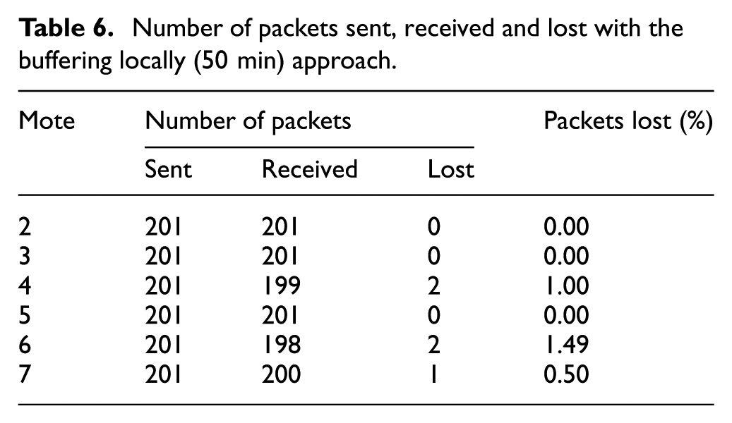
When analysing the number of packets sent, received and lost by each protocol, we will concentrate on the same 7-day period (14 March 2016 to 21 March 2016) for all three approaches. Nodes 0 and 1 only act as relays to forward the data collected and do not generate packets themselves. Table 4 shows the number of sent packets by each node in the ‘send always’ approach, the number of packets that successfully arrived at the sink and the number of lost packets.Tables 5 and 6 show the same data for the two buffering locally approaches. The percentage of lost packets is lower with the buffering locally approaches, especially in the 50-min configuration. It must be noted that in 10-min buffering locally deployment, mote 7 that caused several resets throughout the test period, caused changes in the route, as number of hops, loss of packets (see Figure 4). With the exception of mote 7, the buffering locally approaches show better reliability and very few dropped packets. Table 7 compares the total number of packets sent with each approach during a period of 7 days. It should be noted though that a dropped packet in the buffering locally approaches means the loss of all data from either a 10- or 50-min period, which is a more serious problem than the loss of individual packets from the send always approach. This possible loss of data forms part of the trade-off between the two approaches: the reduction in energy consumption and increased lifetime at the cost of losing small amounts of data.

Table 4.

Number of packets sent, received and lost with the send always approach.

Mote	Number of packets			Packets lost (%)
Mote	Sent	Received	Lost	Packets lost (%)
2	20,160	20,081	79	0.39
3	20,160	20,106	54	0.27
4	20,160	20,113	47	0.23
5	20,160	17,342	2818	13.98
6	20,160	20,104	56	0.28
7	20,160	20,114	46	0.23

Table 5.

Number of packets sent, received and lost with the buffering locally (10 min) approach.

Mote	Number of packets			Packets lost (%)
Mote	Sent	Received	Lost	Packets lost (%)
2	1008	1008	0	0.00
3	1008	1008	0	0.00
4	1008	1005	3	0.30
5	1008	1008	0	0.00
6	1008	1008	0	0.00
7	1008	915	93	9.23

Table 6.

Number of packets sent, received and lost with the buffering locally (50 min) approach.

Mote	Number of packets			Packets lost (%)
Mote	Sent	Received	Lost	Packets lost (%)
2	201	201	0	0.00
3	201	201	0	0.00
4	201	199	2	1.00
5	201	201	0	0.00
6	201	198	2	1.49
7	201	200	1	0.50

Figure 4.

Change in source–destination hop count for mote 7, buffering locally (10 min) approach.

Table 7.

Number of packets sent, lost (%) and drop voltage (volts) lost for each approach.

Approach	Packets sent	Lost (%)	Drop voltage
30 s	120,960	2.56	0.038
10 min	6048	1.59	0.033
50 min	1206	0.50	0.020

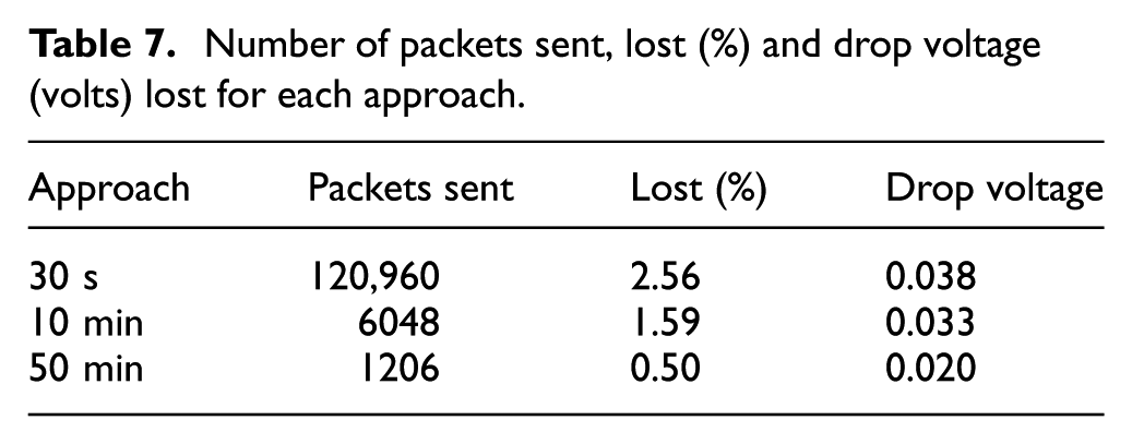
The average voltage for the motes in each deployment is shown in Figure 5, including their standard deviation. The motes use 2 × 1.5 V new AA batteries with 1500 mAh. In the ‘send always’ approach, the voltage dropped 0.038 V; in the ‘buffering locally’ approach, the voltage dropped 0.033 and 0.02 V for 10 and 50 min, respectively. With longer deployments, it is expected that there will be noticeably less drop in voltage with the ‘buffering locally’ approaches than with the ‘send always’ approach. In addition, we can see that the average voltage in ‘send always’ has a shorter standard deviation that means that the behaviour is similar among the motes when the number of sent packets increases. However, in 10 min ‘buffering locally’, these differences are higher, but in 50 min ‘buffering locally’, due to the reduced number of sent packets, showing lower standard deviations.

Figure 5.

Average battery voltage for the different approaches (‘send always’, ‘buffering locally’ for 10 and 50 min) with standard deviations.

The path to the sink used by each mote depends on the considered approach. The larger packet sizes in the ‘buffering locally’ approaches cause variations in the ETX metric used by CTP to determine the best path. We can analyse the number of hops in all source–destination paths in each network. Figure 4 shows how the source–destination path from one mote to the sink changes with time, over a period of 24 h. In this case, the plot corresponds to mote 7 in the network using the buffering locally (10 min) approach. Figures 6 –8 show the distribution of hop counts due to the multihop routing protocol during a 7- day period for all motes in each of the three networks. We can see from these three figures that in the ‘send always’ approach, paths with higher hop counts are used more often than in the ‘buffering locally’ approaches. This is justified because in ‘buffering locally’, we send less packets, the network is less congested and CTP is more stable. This indicates that a shorter, more suitable path to the destination can be found more often in the ‘buffering locally’ approach. Fewer hops also result in less packet forwarding by the nodes in the path, reducing overall radio usage and energy consumption. Lower hop counts also reduce the possibility of losing packets, as each time packet must be forwarded there is a possibility loose the packet due to full queue buffers, interference, network congestion or other factors.

Figure 6.

Distribution of hop counts for each mote, sending always approach.

Figure 7.

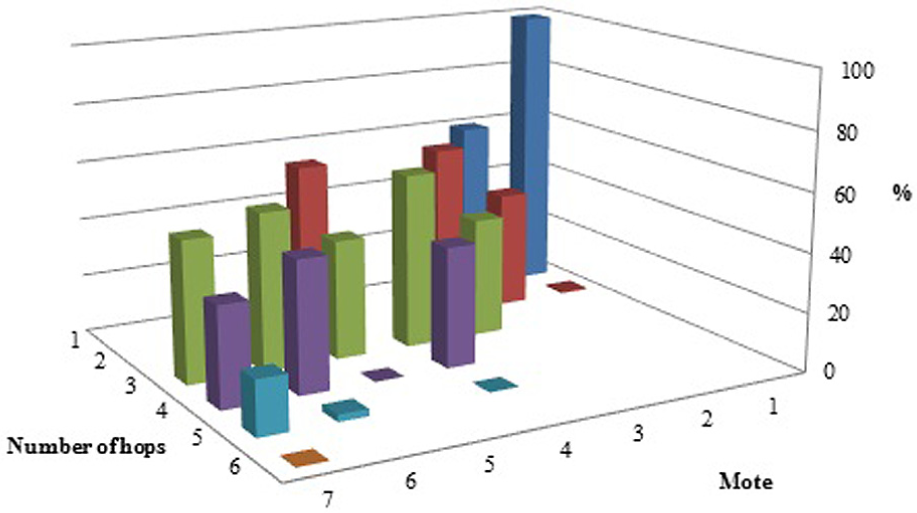
Distribution of hop counts for each mote, buffering locally (10 min) approach.

Figure 8.

Distribution of hop counts for each mote, buffering locally (50 min) approach.

Conclusion

From the results, we conclude that the ‘send always’ approach requires a greater demand in the network due to a much larger number of packets to be sent, which in turn causes a higher energy consumption and shortens the network lifetime. However, one advantage of this approach is that the loss of one or more packets does not necessarily affect the final data gathering. Unless all 20 samples from a 10-min period are lost, there will be always at least one sample in order to estimate the average T and RH for that period.

Finally, with the buffering locally approach, the loss of one packet with 10 or 50 samples avoids estimating these averages. Nevertheless, the main advantages of this approach are the reduced number of packets sent over the network and a larger network lifetime. In this approach, it is strongly recommended to forward a packet at least twice to improve reliability.

Footnotes

Acknowledgements

S.F-C., J.J.P-S. conceived and designed the network and the experiments for data collection; J.S-G., M.G-P. and A.S-A. performed the experiments; S.F-C. and J.S-G. analysed the data and made all the statistical analysis; S.F-C. and J.J.P-S contributed with the WASN nodes; S.F-C. wrote the paper. Copyright © 2017 SAGE Publications Ltd, 1 Oliver’s Yard, 55 City Road, London, EC1Y 1SP, UK. All rights reserved.

Handling Editor: Miguel A Zamora

Declaration of conflicting interests

The author(s) declared no potential conflicts of interest with respect to the research, authorship, and/or publication of this article.

Funding

The author(s) disclosed receipt of the following financial support for the research, authorship, and/or publication of this article: This work was supported by the Universitat de València under the projects UV-INV-PRECOMP14-207134, UV-INVAE15-339582, UV-SFPIE RMD17, by the Generalitat Valenciana under the project GV-2016-002 and mainly by Ministry of Economy and Innovation under the project BIA2016-76957-C3-1-R.

ORCID iD

Jaume Segura-Garcia

References

Jennehag

Forsstrom

Fiordigigli

. Low delay video streaming on the Internet of Things using Raspberry Pi. Electronics 2016; 5: 60.

IEEE 802.15.4:2006. IEEE standard for information technology – telecommunications and information exchange between systems – local and metropolitan area networks – specific requirements – part 15.4: Wireless Medium Access Control (MAC) and Physical Layer (PHY) specifications for Low-Rate Wireless Personal Area Networks (WPANs) (Technical report, 2006).

TelosB datasheet, http://www.memsic.com

Polastre

Szewczyk

Culler

. Telos: enabling ultra-low power wireless research. In: Proceedings of the 4th IEEE international symposium on information processing in sensor networks, Boise, ID, 15 April 2005. New York: IEEE.

TinyOS, https://github.com/tinyos/tinyos-main

Levis

Madden

Polastre

et al . TinyOS: an operating system for sensor networks. In: Weber

Rabaey

Aarts

(eds) Ambient intelligence. Berlin; Heidelberg: Springer-Verlag, 2005, pp.115–148.

Strazdins

Elsts

Nesenbergs

et al . Wireless sensor network operating system design rules based on real-world deployment survey. J Sens Actuator Netw 2013; 2(3): 509–556.

Delamo

Felici-Castell

Pérez-Solano

et al . Designing an open source maintenance-free Environmental Monitoring Application for Wireless Sensor Networks. J Syst Software 2015; 103: 238–247.

Xing

et al . Optimal sensor placement and measurement of wind for water quality studies in urban reservoirs. In: Proceedings of the ACM/IEEE 13th international symposium on information processing in sensor networks (IPSN), Berlin, 15–17 April 2014, pp.167–178. New York: IEEE Press.

10.

Corke

Wark

Jurdak

et al . Environmental wireless sensor networks. P IEEE 2010; 98(11): 1903–1917.

11.

Lim

Woehrle

Meier

et al . Harvester – energy savings through synchronized low-power listening. In: Proceedings of the 6th European workshop on sensor networks, Cork, 11–13 February 2009, pp.29–30. ACM.

12.

EPA. Quality assurance handbook for air pollution measurement systems – volume IV: meteorological measurements version 2.0. Technical report EPA-454/B-08-002, March 2008, https://www3.epa.gov/ttnamti1/files/ambient/met/Volume_IV_Meteorological_Measurements.pdf

13.

Burri

Von Rickenbach

Wattenhofer

. Dozer: ultra-low power data gathering in sensor networks. In: Proceedings of the 6th IEEE international symposium on information processing in sensor networks, Cambridge, MA, 25–27 April 2007, pp.450–459. New York: IEEE.

14.

Ingelrest

Barrenetxea

Schaefer

et al . SensorScope: application-specific sensor network for environmental monitoring. ACM T Sensor Network 2010; 6: 17.

15.

Liu

et al . Does wireless sensor network scale? A measurement study on GreenOrbs. IEEE T Parall Distr 2013; 24(10): 1983–1993.

16.

Fonseca

Gnawali

Jamieson

et al . TEP 123: the collection tree protocol (CTP). TinyOS 2.0.2 documentation, February 2007, http://tinyos.stanford.edu/tinyos-wiki/index.php/TinyOS_Network_Protocol_Working_Group

17.

Gallart

Felici-Castell

Delamo

et al . Evaluation of a real, low cost, urban WSN deployment for accurate environmental monitoring. In: Proceedings of the 2011 IEEE 8th international conference on mobile adhoc and sensor systems (MASS), Valencia, 17–22 October 2011, pp.634–639. New York: IEEE.

18.

Aguirre-Guerrero

Marcelín-Jiménez

Rodriguez-Colina

et al . Congestion control for a fair packet delivery in WSN: from a complex system perspective. Sci World J 2014; 2014: 381305.

19.

Yang

Z-L

Min

H-Q

. Deployment of wireless sensor networks for oilfield monitoring by multiobjective discrete binary particle swarm optimization. J Sensors 2016; 2016: 9358358.

20.

Gana Kolo

Anandan Shanmugam

Gin Lim

et al . An adaptive lossless data compression scheme for wireless sensor networks. J Sensors 2012; 2012: 539638.

21.

Zennaro

Ntareme

Bagula

. Experimental evaluation of temporal and energy characteristics of an outdoor sensor network. In: Proceedings of the international conference on mobile technology, applications & systems, Yilan, Taiwan, 10–12 September 2008. New York: ACM.

22.

Mathur

Desnoyers

Chukiu

et al . Ultra-low power data storage for sensor networks. ACM T Sensor Network 2009; 5(4): 33.

23.

Pérez-Solano

Felici-Castell

. Improving time synchronization in Wireless Sensor Networks using Bayesian Inference. J Netw Comput Appl 2017; 82: 47–55.

24.

Moss

Hui

Klues

. TEP 105: low power listening. TinyOS 2.0.2 documentation. Technical report, 2008, http://tinyos.stanford.edu/tinyos-wiki/index.php/TEPs

25.

Ogawa

de Oliveira

Rodrigues

et al . Energy consumption and memory footprint evaluation of RPL and CTP in TinyOS. In: Proceedings of the XXXIV Simposio Brasileiro de Telecomunicaçoes (SBrT 2016), Santarém, PA, 30 August–2 September 2016, http://sbrt.org.br/sbrt2016/anais/ST02/1570270153.pdf (accessed 14 March 2018).

Experimental trade-offs between different strategies for multihop communications evaluated over real deployments of wireless sensor network for environmental monitoring

Abstract

Keywords

Introduction

Related works

Hardware and software: TelosB and TinyOS

TelosB mote

TinyOS

Design issues for EM applications

Send always versus buffering locally

Analysis and evaluation of send always and buffering locally approaches under a real WSN deployment

Description of the deployment

Performance evaluation metrics

Results

Conclusion

Footnotes

Acknowledgements

Declaration of conflicting interests

Funding

ORCID iD

References