Real-time predication and navigation on traffic congestion model with equilibrium Markov chain

Abstract

With the explosive growth of vehicles on the road, traffic congestion has become an inevitable problem when applying guidance algorithms to transportation networks in a busy and crowded city. In our study, the authors proposed an advanced prediction and navigation models on a dynamic traffic network. In contrast to the traditional shortest path algorithms, focused on the static network, the first part of our guiding method considered the potential traffic jams and was developed to provide the optimal driving advice for the distinct periods of a day. Accordingly, by dividing the real-time Global Positioning System data of taxis in Shenzhen city into 50 regions, the equilibrium Markov chain model was designed for dispatching vehicles and applied to ease the city congestion. With the reveals of our field experiments, the traffic congestion of city traffic networks can be alleviated effectively and efficiently, the system performance also can be retained.

Introduction

Traffic congestion is a common phenomenon which may cause serious consequences, such as economic loss, additional delay, and air pollution. Traditionally, the growth of traffic congestion was considered as the result of unsuitable land use, the shortfall of roadway capacity, the growth of vehicular traffic volume, inappropriate infrastructure supply, and so on. ¹ To alleviate congestion and reduce losses, an intelligent method of measuring traffic jam and navigating the available road should be used in the current transportation system.

Many practical vehicle navigation algorithms are therefore proposed to tackle routing problems in the traffic condition changing in real-time condition. For example, pioneering work by Cooke and Halsey ² has studied shortest path algorithms on a time-dependent network. Since then, such kinds of problems have attracted many researchers’ attention.

In our study, the authors collected the taxi routing information in Shenzhen city, China, and proposed the newly real-time predication and navigation system on the dynamic city transportation network to solve the problem in Shenzhen city. Compared to Ahuja et al.’s solution in 1993, which is derived from the static transportation network, our proposed method takes the complicated and dynamic road condition into account and outperforms on the field experiments.

Depending on our observation, the traffic congestion exerts a tremendous influence on the city transportation. Our system can adaptively update systems prediction of the traffic jam. Moreover, a newly congestion prediction and alleviation algorithm was proposed by the idea of Markov chain with the consideration of state changing. To be specific, the collected Global Positioning System (GPS) information of Shenzhen taxi portioned into 50 groups by the transferring probability matrix. With the derivation of the matrix, our system can predicate the traffic condition, and the equilibrium state also can be computed with the progress of Markov chain. Beyond that, the travel time of each road was divided into distinct periods and used for constructing a dynamic transportation network for navigation in Shenzhen. The main contributions of this article are listed as follows:

1. In the navigation part, the authors proposed a method that can solve the time-dependent network routing problem, and the derived navigation path can be updated timely by referring the traveling time arrangement.

2. In the prediction part, the equilibrium Markov chain was proposed to handle the traffic congestion condition by the traffic states computation. That is, the congestion alleviation strategy is designed to balance the equilibrium states via the computation of Markov transferring probability matrix.

The remainder of this article is organized as follows. The related work on transportation routing networks is presented in section “Related work.” Section “Dynamic transportation network” discusses data preprocessing strategy and city transportation network constructed by the basic vehicle data. Section “New time-dependent navigation algorithm” presents the design of the routing algorithm in detail. The Markov chain model is shown in section “City modeling,” including vehicles clustering, transferring probability matrix, and equilibrium states. Section “New congestion alleviation algorithm” describes the congestion alleviation strategy and model verification. In section “Case study,” a case study is carried out and our method is evaluated. Finally, section “Conclusion” concludes the article and reiterates the contributions.

Related work

With the fateful consequences caused by traffic congestion, a growing number of researchers show solicitude for techniques of navigating on a dynamic network where congestion happened. Dreyfus, ³ Ahuja et al., ⁴ and Bast et al. ⁵ have given a detailed review of the transportation routing literature and introduced a couple of methods based on the shortest path algorithm. Their work shows that the literature on finding the shortest or fastest path is vast with several attempts made to find the minimum cost path on a time-dependent network.

According to some researchers, the time-dependent navigation problem is a generalization of the traditional shortest path problem with a dynamic network that travel times change over time. LeBlanc et al. ⁶ considered the road cost variation and presented a solution to the transportation system with nonlinear road costs. Ziliaskopoulos and Mahmassani ⁷ developed an algorithm depending on general Bellman’s principle of optimality to calculate dynamic costs. Designed for intelligent transportation systems where real-time information is available, optimal adaptive routing algorithms were proposed by Kaufman and Smith ⁸ and Fu. ⁹ Other than making improvements in traditional algorithms, the stochastic ways of tackling methods were addressed by Pearl, ¹⁰ Chabini and Lan, ¹¹ Ardakani and Tavana. ¹² They used heuristic methods like A* or tabu search to find the optimal solutions to such problems. Similarly, Bell and McMullen ¹³ thought that the procedure of vehicle routing simulates the process of ants foraging for food and applied ant colony optimization techniques to the traffic network.

In addition to the efforts by researchers who want to find out navigation algorithms on a traffic network where congestion is likely to appear, a significant number of them also hope to seek out when congestion happens. To detect traffic jams, Sun et al. ¹⁴ used the possibility theory and support vector machines (SVMs) to forecast traffic congestion, while Lei et al. ¹⁵ developed a method to extract jam events by analyzing the road background feature using multiple background images. Furthermore, a traffic jam detection framework was designed by Gupta et al., ¹⁶ using data from all kinds of GPS-enabled devices such as mobiles and tablets from vehicles. This framework has the ability to detect areas where traffic congestion frequently occurs. Awan and Rani ¹⁷ proposed a technique to process digital data to estimate traffic density directly from video images in real time.

Based on some work that has tried to construct a traffic model and predict congested situations, a further step has been taken to provide routing strategy and avoid traffic congestion. Asif et al. ¹⁸ introduced a variable window-support vector regression (SVR) method for predicting vehicle speed over an artificial neural network (ANN). This method can be utilized for route guidance and congestion avoidance. Kim and Kang ¹⁹ implemented a route determining method that provided the adaptive routes for traffic conditions, as well as scalable routing services for users’ preferences. Hu et al. ²⁰ presented a model that could be applied to the dynamic strategy of traffic lights to improve traffic flow in cities. A protocol introduced by Hussain et al. ²¹ suggested a way to guide vehicles to their destinations while managing congestion and avoiding deadlock situations in urban city grids. Miller-Hooks and Mahmassani ²² assumed that travel time of an arc could be known as a priori knowledge. Sachdeva et al. ²³ attempted to develop a multiagent-based real-time centralized evolutionary optimization technique for managing urban traffic by controlling traffic signals.

Inspired by their work and combined with our navigation algorithm and prediction model, we derived a simple but efficient strategy that guides vehicles and alleviates traffic congestion in our field study.

Dynamic transportation network

To consummate the city transportation network, a prerequisite for advanced research, such as dynamic navigation path algorithm and the behavior modeling of vehicles, congestion prediction should be first built. In our study, we installed GPS devices on taxis in Shenzhen city to construct a vibrant city transportation network, from 15 June to 16 July in 2015. Large-scale GPS dataset was acquired from approximately 20,000 taxis and stored in PostgreSQL with a spatial database extension called PostGIS. Real-time taxi information was collected in the format of longitude/latitude, time stamps, passenger status (i.e. occupied or vacant), driving speed, and orientation. The data were uploaded to the central server via telecommunication network at a sampling rate of four times per minute.

Data cleaning

For reasons of device error or poor network connection, the collected raw data could contain some mistakes for further use, hence the procedure of data cleaning is needed. In the beginning, abnormal points were detected with characteristics of being far away from Shenzhen city boundary or possessing exceedingly high speed. Such instances normally lie in network transfer deviation or device error. Consequently, we filtered out exceptional taxi records that were out-of-bounds or reached speeds that were 10 times higher than 150 km/h.

To relieve the computation from tolerance error of GPS device, we expanded the boundary of Shenzhen by 1 km, as illustrated in Figure 1. The result area is described as the buffered region and GPS points that are out of this region are regarded as invalid and will be cleaned.

Figure 1.

Overview of before and after expanding the city boundary in Shenzhen city.

Swing data handling

The authors sorted the data points of every taxi by time and linked up with adjacent points belonging to each taxi, as shown in Figure 2. According to this figure, attention should be paid to abnormalities, such as bunches of conflicting data swinging between roads, which are possibly due to the error from GPS data. For this problem, our solution is derived from the analysis of empirical cumulative distribution function. The GPS data of each taxi was sorted by time in Figure 3(a).

Figure 2.

The GPS point swing between road A and road B. This means the trace routes on roads A and B happened at the same time.

Figure 3.

The empirical cumulative distribution functions on time interval between (a) two neighboring points in a trace and (b) on the speed of taxi points.

Depending on the illustration, about 95% of time intervals between two locating points are smaller than 120 s. Thus, it is more probable that the GPS device is broken or the driver idles on this route if the time interval between two neighboring points is larger than 120 s. In this case, the data route will be considered as a new trip for this taxi. On the other hand, the taxi speed is hardly above 96 km/h, which can be observed from Figure 3(b). Our system split the point traces into two sequences in the event of distance between adjacent data points being greater than 3200 m. Finally, the eliminated traces were lesser than 1300 m or contained less than 10 points. For example, in our experiment, 16 million records are filtered from 19.5 million raw records.

Dynamic network construction

Accordingly, GPS location and speed status for each taxi can be categorized into every moment of every day. Vehicles trace can be easily calculated by connecting each GPS dots in time-ordered sequence. Figure 4 shows four traces of one vehicle at the distinct time in 1 day (15 minimum time periods per figure). Each trace route consisted of four colors to indicate the different speeds, that is, green for fast, yellow for normal, orange for slow, and red for very slow, respectively. Moreover, main roads were referred as the leading city transportation network. By recording the speed and GPS location of each vehicle, the average speed in the period of driving time can be easily mapped to the general vehicles speed to the nearest roads. Figure 5 shows the average speed on the main road at a period in 1 day. It represents some parts of the entire transportation network of Shenzhen City. Similar to Figure 4, distinct colors stand for different mean speeds. The current setup of city transportation network makes it easy to indicate the city traffic dynamically with the mean speed of each road.

Figure 4.

Taxi trace routes at 15-min time period within 1 day.

Figure 5.

Dynamic city transportation network with four different periods of time within 1 day.

New time-dependent navigation algorithm

Accordingly, the city transportation network was defined by a graph with arcs representing roads and nodes indicated by intersections. For a real-world routing problem, road conditions change and traffic congestion may occur at a certain time on roads. Our system consisted of the navigation and prediction models. In the first section, the time-dependent navigation model is proposed, which tackles problems on the dynamic transportation network and finds the optimal navigation routing path for the given destination.

Definitions and notations

Let $G=(N,E,D,C)$ be a directed network where $N=\{1,...,n\}$ is a set of nodes and $E=\{(i,j)\in N*N\}$ is a set of arcs. $D=\{d_{\mathrm{ij}}(t)|(i,j)\in E\}$ is used to describe the set of time-dependent arc travel times and $C=\{{\mu }_{\mathrm{ij}}(t)|(i,j)\in E\}$ is represented as a set of time-dependent arc travel costs. ${\mu }_{\mathrm{ij}}(t)$ is the mean travel time (cost) of arc $(i,j)$ at t. The mean travel time from nodes i to j is assumed to be available at any time. Such information is calculated from the taxi data of Shenzhen city and time t is considered to be in a certain time interval. From 1-day midnight till the ensuing days, time is divided into 96 periods, every 15 min, like $(00:00~00:15)$ , $(00:15~00:30)$ , $(00:30~00:45),...$ , and each period is called a time interval. Specifically, the road is assumed to maintain the same driving speed as long as it is in the identical interval. As a result, asking for the value of ${\mu }_{\mathrm{ij}}(t)$ actually includes two steps of work. First, find out the time interval that t is counted in, then query the mean travel time from nodes i to j at this time interval. For instance, to get the value of ${\mu }_{1,5}(15:32)$ , we first check out that $(15:32)$ is in interval $(15:30~15:45)$ , and then derive the result of speed from node 1 to node 5 in this interval.

First-in-first-out assumption

The transportation network was assumed by the following first-in-first-out (FIFO) condition. According to the literature, Dean ²⁴ and Dehne et al. ²⁵ proposed the time-dependent network under the FIFO method, not only because many networks had this particular characteristic in practice, but also because under this assumption, time-dependent shortest path problems exhibited many friendly structural properties.

Intuitively, the FIFO condition stipulates that vehicles exit from an arc in the same order as they entered, so that a later-entered vehicle never results in an earlier arrival at the endpoint of an arc. For a mathematical description, the FIFO condition is valid if and only if the following inequality is satisfied

$$t+{\mu }_{ij}(t)\le (t+1)+{\mu }_{ij}(t+1),\forall (i,j,t)$$

(1)

When the FIFO condition holds by this equation, the transportation network is testified and is reliable.

Algorithm description

Figure 6 illustrates a network example with 6 nodes (n = 6) and 8 arcs (m = 8). There are four paths from origin node 0 to destination node 5: 0-2-4-5, 0-2-5, 0-1-3-4, 0-1-5. Figure 6(a) shows the circumstances in a static network that the cost of each arc is constant. The red line indicates the derived path of the shortest path problem based on the navigation algorithm. The driving cost may change due to the discrepancy in traffic conditions.

Figure 6.

Routing path with (a) time-independent network and (b) time-dependent network.

A preeminent algorithm is supposed to find an optimal path according to dynamically updated link travel time. As shown in Figure 6(b), we departed from node 0 at time t and then at arrival of node 1, the travel time of $t\prime$ starting from node 1 will be taken into account. Arc (1,5) is chosen as a new path on the optimal result. The reason (1,3,5) was not considered as the result could be due to the congestion occurrence on the link with time $t\prime$ or $t″$ .

The target function could be expressed by a recursive equation. Suppose we start from origin p at time t and aim at getting to destination q. $\mathrm{out}(i)$ is defined as the set of destination nodes directly connected to the starting node i. Besides, ${\pi }_i(t)$ is designed to be the fastest travel time to destination q departing from node i at time t. The time-dependent navigation problem can be defined as follows

$${\pi }_i(t)=\{\begin{array}{cc}\underset{j\in \mathrm{out}(i)}{min}\{{\mu }_{\mathrm{ij}}(t)+{\pi }_j(t+{\mu }_{\mathrm{ij}}(t))\},\hfill & i\ne q\hfill \\ \multicolumn{1}{c}{0,}& i=q\hfill \end{array}$$

(2)

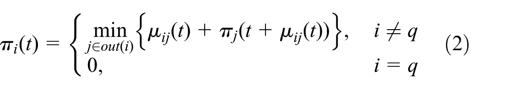
In conformity with equation (2), a decision was made at node i to determine which adjacent node j should be chosen to have a minimum traveling time from node i to destination node. Hence, our goal tries to find the solution of $\pi (t_0)$ heuristically.

A straightforward approach to find the shortest time path from current node to destination node was to directly update all the connected nodes and move toward the destination with repeated iterations. It should be noted that the network size decreases as the driver travels toward the terminal point and, consequently, the optimization process becomes faster. Because of the assumption that the transportation network satisfied the FIFO condition, nodes related to time t will never be used to update nodes corresponding to times greater than t. In other words, the optimal navigation path can be set in decreasing order of departure time periods. The proposed method is presented in Algorithm 1.

Algorithm 1. Time-dependent navigation algorithm

Input: All nodes: $N$ , Start Node: $p$ , End Node: $q$ , Start Time: $t$ , Nodes starting from $i:\mathrm{out}(i)$ Output: travel time from $p$ to $q$ 1:  $\mathrm{Queue}\leftarrow \varphi \cup \{(p,t)\}$ 2:  While $\mathrm{current}\_\mathrm{node}$ is not $q$ do 3:     ▹Get a pair from Queue with minimum time 4:    $(\mathrm{current}\_\mathrm{node},\mathrm{current}\_\mathrm{time})\leftarrow \mathrm{Queue}$ . 5:   for $j\in \mathrm{out}(\mathrm{current}\_\mathrm{node})$ do 6:    if $j$ is non-essential then 7:      $N\leftarrow N-j$ ▹Remove j from N 8:    end if 9:      ▹from current_node to j at current_time 10:     $\mathrm{new}\_\mathrm{time}\leftarrow \mathrm{arrival}\_\mathrm{time}$ 11:     $\mathrm{Queue}\leftarrow \mathrm{Queue}\cup \{(j,\mathrm{new}\_\mathrm{time})\}$ 12:   end for 13:  end while 14: return $\mathrm{current}\_\mathrm{time}$

As described in step 3 of Algorithm 1, the size of the network was determined by evaluating non-essential nodes. Here, the authors define non-essential nodes as the nodes that are unlikely to be on the optimal route. The intuition is that opportunities to find a possible plan through backward node are vague. For a navigation problem, we should approach the destination at each iteration in an ideal condition. Considering that modest deviation is acceptable in practical problems, we used the following simple function to judge whether a node was essential

$$\sigma (j)=\omega *d_{j}q(t)-d_{i}q(t)$$

(3)

Node j is considered essential if $\sigma (j)$ is less than 0. Otherwise, it is regarded as the non-essential value and is deleted from the network. The algorithm converges with time complexity $O(\mathrm{kmn}\log (n))$ .

City modeling

In the previous section, we applied a time-dependent navigation algorithm, which made vehicle navigation more intelligent and efficient on the dynamic transportation city network. Meanwhile, city congestion is a pivotal part of urban transport. To figure out congestion in the current transportation system, in our study, the equilibrium Markov chain model was applied to dispute the movements of vehicles and derived as strategies for alleviating traffic congestion.

Area clustering

First, our system divided GPS locating areas into diverse groups. Due to the movement of vehicles, the Euclidean distance of latitude and longitude calculated from the GPS data was recorded and presented as the transferring probability matrix based on these groups. Besides, our system used the k-means clustering algorithm, which costs less time at computing and produces reliable clustering results. Unfortunately, there is no consensus on how to find the best values for the number of cluster parameters (i.e. k value) in k-means for a given problem. Intuitively, this parameter can be empirically chosen according to the specific regionalism architecture of the city (including commercial zone, residential zone, industrial zone, etc.). In our experiment, the number is empirically set to 50 according to the suggestion of the Shenzhen city traffic department, which gives promising results. Specifically, our system takes 90 min to partition 16 million GPS points into 50 clusters. Figure 7 is the referring example. It represents three distinct results after 500 iterations with k-means algorithm. The total squared errors in Figure 7(a)–(c) are 6644.754, 5718.202, and 5766.307, respectively. Since Figure 7(b) shows the smallest obtained summarized squared errors in our example, we use the partitioned result of 50 clusters in our system.

Figure 7.

The city is divided into 50 regions generated by k-means algorithm (after 500 iterations) according to taxi GPS data. (a), (b), and (c) represent the clustering results with three different random seeds.

Traffic transfer matrix

$$\left[\begin{array}{ccc}{m}_{1,1}\hfill & \cdots \hfill & m_{1,50}\hfill \\ \multicolumn{1}{c}{⋮}& \ddots \hfill & ⋮\hfill \\ \multicolumn{1}{c}{m_{50,1}}& \cdots \hfill & m_{50,50}\hfill \end{array}\right]$$

(4)

Equation (4) is the transferring probability matrix of 50 clusters and it is recollected for every half-hour. During this half-hour, if a vehicle moved from cluster i to cluster j, $m_{i,j}$ would be plus 1. After traversing all the vehicles in that half-hour, the transferring probability matrix was normalized by the sum of every row, which guaranteed the convergence and existence of an equilibrium state. According to our example, a total of 1536 transferring probability matrices in 32 days were worked out for the derivation in the following section.

Equilibrium state

Equation (5) is the statement of the equilibrium state, where ${\pi }^T$ is the equilibrium distribution and P is the transferring probability matrix defined previously. No matter how many times inter-region transfers happen in the future, ${\pi }^T$ does not change anymore. That is

$${\pi }^{T}P={\pi }^T$$

(5)

where $\pi$ is a row eigenvector of matrix P if $\sum _{i=1}^N{\pi }_i=1$ and ${\pi }_i>0$ for all i holds. As a consequence, equilibrium state can be obtained even more quickly.

Algorithm 2 is the pseudocode of the equilibrium state. In practice, this state converges reasonably quickly while the general processes keep stable in 50 loops. According to the definition of the equilibrium state in our study, the tendency and following location of the vehicle in Shenzhen city can be computed, and the jammed condition of the region even can be predicted in contrast to the present time.

Algorithm 2. Equilibrium state generation.

Input: $\mathrm{initialState},\mathrm{transferMatrix}$ Output: $\mathrm{steadyState}$ 1:  function SEARCH $(\mathrm{initState},\mathrm{transferMatrix})$ 2:    $\mathrm{maxDistance}\leftarrow 1000$ 3:    $\mathrm{steadyState}\leftarrow \mathrm{initialState}$ 4:   while $\mathrm{maxDistance}>0.5$ do 5:     $\mathrm{state}\leftarrow \mathrm{steadyState}*\mathrm{transferMatrix}$ 6:     $\mathrm{all}\_\mathrm{distance}\leftarrow \parallel (\mathrm{state}-\mathrm{steadyState})\parallel$ 7:     $\mathrm{maxDistance}\leftarrow max(\mathrm{all}\_\mathrm{distanc})$ 8:     $\mathrm{steadyState}\leftarrow \mathrm{state}$ 9:   end while 10:  return $\mathrm{steadyState}$ 11:  end function

New congestion alleviation algorithm

Congestion measuring

In this section, we aimed to measure the congestion of a cluster of the equilibrium states of Markov chain. Estimated from the number of vehicles, driving speed and location were considered and exploited to judge congestion. Roads in the city were variable in the width and vehicle capacities, hence, to measure the congestion degree in an area, it was reasonable to find out a correlation between the speed and number of vehicles for every cluster. First, we filtered out the road without any vehicles to reduce the computational burden. We approximated the correlation function with the numbers of vehicle and the related speed (Figure 8). Investigating from our field experiments, although there existed some randomness situations in the sparse vehicles area, the relation still can be interpreted by the sigmoid curve. Such sigmoid-like curve is represented as the speed of vehicles in the congested area by giving the number of vehicles, which was defined as follows

$$S=\frac{\alpha }{\beta +e^{\lambda (N-ϵ)}}$$

(6)

where N is the number of vehicles and S is the average speed of the cluster. Constant variables of $\alpha$ , $\beta$ , $ϵ$ , and $\lambda$ were distinct in different clusters and were determined using data fitting.

Figure 8.

The fitted curve and scatter of the relation between number of vehicles (x-axis) and average speed (y-axis) of one cluster. In this cluster, $\alpha =2595$ , $\beta =63.14$ , $\lambda =1879.0$ , and $ϵ=0.001407$ after fitting.

Vehicle guiding system

To evaluate the traffic network, the following equation was used to weight the speed

$$S_{\omega }=\sum \frac{N_i}{N}{S}_i$$

(7)

$S_i$ is defined as the average speed calculated from equation (6), $N_i$ is represented as the number of vehicles in cluster i, and N refers to the total number of vehicles. According to Bast et al., ⁵ if the average speed is less than 20 km/h for each vehicle, this area/cluster will be regarded as congested and our guiding strategy will be applied to ease this situation.

According to the equilibrium state, when the $S_{\omega }$ value is larger than 20 km/h, our system would adopt sequential minimal optimization (SMO) method, which was introduced by Platt, ²⁶ to adjust the transferring probability matrix to alleviate the congestion situation in the area. SMO method provided an efficient way to solve the optimization problem by interactively breaking the problem into a series of smallest possible subproblems, and solving them analytically. The following procedures started at the most congested cluster and applied to the next cluster sequentially:

1. Sort the average speed of vehicles for each cluster and find the smallest speed in cluster $C_i$ .

2. Via the transferring probability matrix, obtain the adjacent clusters $C_{\mathrm{adjacent}}$ .

3. Decrease the probability $m(\mathrm{adjacent},i)$ until $S_w$ in the adjusted equilibrium state reaches its minimum value.

4. If we update the value of $m(\mathrm{adjacent},i)$ , on the contrary, the other probabilities in a row should be renormalized to 1 again.

5. Repeat the procedure until $S_w$ is convergent and larger than 20 km/h.

Before the system applies it, there are two restrictions: (1) after system implementation, the alleviate method would reduce the number of vehicles in the congested cluster. The greater number of the reducing vehicles could make the larger adjustment in the real-life traffic network. In our case, 30% reducing rate can be observed from the practical case and (2) in our study, the transferring probability between two nonadjacent clusters cannot be changed. The value was set to 0 in the matrix.

Case study

This section describes a case study conducting our time-dependent algorithm on the districts of Shenzhen city, where the traffic congestion problem is a serious concern that happens all the time. According to our previous assumption, this area was depicted as a network with nodes connected with directed arcs corresponding to the intersections and road situations in real traffic. Besides, the taxi data was used to derive at the road distance as well as the real-time traffic flow information.

Comparison of navigation algorithms

Our first experiment was proposed to test the selected route with a different time for every 15-min intervals. In total, 96 time periods, in 1 day, were calculated by our collecting data; the results are illustrated in Figure 9. A conclusion easily drawn from the figure was that traffic congestion does happen to the navigation route in two time periods, around 8 am and 5 pm, evidently a longer time needed to pass through this road section.

Figure 9.

Routing time of the same path in different time intervals, respectively. The x-axis indicates different time intervals within 1 day, while the y-axis represents the total routing time cost.

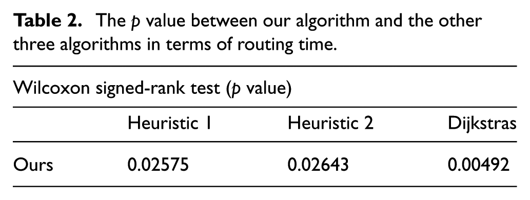
Accordingly, to testify the ability of our proposed time-dependent navigation algorithm, we compare our newly proposed algorithm with the traditional shortest-path algorithm named Dijkstra and two other heuristic time-dependent algorithms, heuristic 1 and heuristic 2, proposed in Wen et al. ²⁷ on several randomly generated circumstances. (For notation convenience, hereafter H1 and H2 are adopted to represent heuristic 1 and heuristic 2, respectively, in Tables 1 and 3.)Table 1 depicts the compared results on the time cost for each algorithm and Figure 10 shows the system execution time for these four methods. Also, nonparametric test Wilcoxon signed rank (WSR) is conducted to further verify the algorithm, whose results are outlined in Table 2. All the p values in Table 2 are less than 0.05, which means that the null hypothesis was rejected and the proposed algorithm indeed differs from other algorithms. Moreover, Table 3 depicts the routing distance of four algorithms, respectively. These comparisons showed that our proposed navigation method could be more accurate and efficient than other navigation solutions in finding the optimal time-saving routing path. Generally, time-dependent methods have good performance with traveling time but very little for the travel distance improvement. Although these two heuristic methods will need extra time cost sometimes, our approach always obtained the equal or lower time cost of routing. Furthermore, Figure 10 indicates that our proposed method has a similar or even less execution time than the other three methods.

Table 1.

Routing time of generated route by each algorithm.

Case	Our method	H1	H2	Dijkstra
1	18.933	19.195	18.933	25.227
2	22.341	22.256	22.342	22.747
3	11.701	11.541	11.724	23.888
4	14.891	15.395	15.016	15.463
5	30.921	31.065	30.921	40.200

Figure 10.

Statistical results of running time of four algorithms, respectively. The x-axis is the index of four algorithms and the y-axis is the running time in microseconds (µs).

Table 2.

The p value between our algorithm and the other three algorithms in terms of routing time.

Wilcoxon signed-rank test (p value)
	Heuristic 1	Heuristic 2	Dijkstras
Ours	0.02575	0.02643	0.00492

Table 3.

Routing distance of generated route by each algorithm.

Case	Our method	H1	H2	Dijkstra
1	20.782	20.494	20.782	18.231
2	17.168	17.019	17.168	17.132
3	15.975	15.823	17.226	15.718
4	27.438	41.292	27.449	27.240
5	24.165	24.251	24.165	24.120

Performance of congestion alleviation algorithm

In this experiment, the authors testified the proposed alleviation strategy referred in the previous section. GPS data from Shenzhen city was first clustered into 50 regions and formulated in a transferring probability matrix for each region by equation (4). When applying our alleviation strategy to the matrix, new equilibrium states were derived as the average speed for each cluster calculated from equation (7). In Figure 11, we reveal two comparison results: the two dotted lines stand for the average speed in each equilibrium state with distinct clusters, the green dotted line is the original data, and the red dotted line represents the adjusting result of our proposed method. With the original taxi data, we can tell the average speed of the taxi speed for 50 clusters ranging from 14 to 40 km/h, which means vehicles moved slowly in some districts and the traffic situation was not good. When we test the same data with our proposed guiding system, the city tended to have a smooth traffic situation, and the cars speed in the low moving districts could be raised up to about 20 km/h. The comparing average speed for all the clusters is between 23 and 25 km/h. The results show that our guiding system could ease or avoid the traffic congestion. Figure 12 also uses the histogram to reveal the cluster counting on the corresponding speed. The left histogram refers to the state with the original traffic situation while the right-hand side figure shows the state solved by our method. According to the figure, the speed distributes around 35 km/h in the original situation, and the average speed applied by our method is 28 km/h. We can tell most of the low-speed districts to improve their average speed after adjustment by our method.

Figure 11.

The average speed of 50 clustered city regions before and after adjustment. The x-axis depicts that the region number ranges from 1 to 50, while the y-axis represents the average speed within each region, respectively.

Figure 12.

Overview of city traffic conditions in terms of average speed of 50 equilibrium states before and after adjustment, respectively. The x-axis represents the average speed and the y-axis shows the number of regions with the corresponding average speed.

Another experiment is shown in Figure 13, which is a comparison of the proportion of the average speed of the equilibrium states. The wider the proportion, the higher is the average speed of the traffic network. The left-hand side figure is the proportion of average speed of 50 clusters in a specific time interval of the city. We can see that some districts have a very minimal average speed in the original states. After applying our guiding method, the districts of low-average decrease and the city has smooth traffic obviously. Besides, the right-hand side figure shows the 1536 equilibrium states during 32 days in Shenzhen city. It was easy to find that the average speed of some equilibrium states was quite low. This may be due to car accidents, weather, or other issues so that the districts with high traffic loading had a very low speed at that data collecting time. After the implementation of our proposed method, most of the equilibrium states have a speed higher than 20 km/h and the traffic problem can be solved.

Figure 13.

The proportion of 50 clustered regions in terms of average speed in the region (before and after adjustment). The y-axis indicates the average speed, while the width of the corresponding area in yellow reveals the number of regions with different average speeds, respectively.

Conclusion

In our study, the authors proposed a time-dependent navigation algorithm to improve driving experience on a dynamic network. With consideration of the constantly changing road conditions, our method improved the travel cost depending on the distance and the time expense in different time periods. Furthermore, an equilibrium Markov-chain-based model was made to ease congestion in the traffic network of Shenzhen city, China. This model was developed to predict congestion of the equilibrium states and alleviate it by a vehicle guiding model. Because the equilibrium state can be derived quickly, the proposed model could provide an effective transferring probability matrix to reflect the real-time congestion situation.

The experimental results demonstrate that our scheme was testified for traffic management. The optimal route was achieved by the navigation algorithm with significant improvement in traveling time, and the Markov chain model also performed well in congestion prediction as well as alleviation.

As the future work, considering the navigation algorithm is built on the transportation network which is built with historic GPS data will undoubtedly be very sensitive to the network status. Further improvement should be focused on the network’s adaptation and robustness. Nowadays, the sharing transporting application, Didi and Uber, are two popular companies in China. It is completely feasible to acquire the real-time GPS location of moving vehicles from Didi’s and Uber’s systems. The authors will also attempt to make the network into real-time self-update so that the Markov model can be more robust.