Sage Journals: Discover world-class research

Abstract

Current experimental investigations on microfracturing (or acoustic emission) events mainly focus on their location and distribution. A new function in rock failure process analysis (RFPA^2D) code was developed to capture the size and number of damage element groups in each loading step. The rock failure process evolving from the initiation, propagation, and nucleation of microcracks was visually simulated by RFPA^2D in this research. Based on the newly developed function, the statistical quantitative analysis of microfracturing events in rock was effectively conducted. The results show that microfracturing (failed element) events in the whole failure process accord with negative power law distribution, showing fractal features. When approaching a self-organized criticality state, the power exponent does not vary drastically, which ranges around 1.5 approximately. The power exponent decreases correspondingly as the stress increases. Through the analysis of the frequency and size of damaged element groups by rescaled range analysis method, the time series of microfracturing events exhibits the self-similar scale-invariant properties. Through the analysis by the correlation function method, the absolute value of the self-correlation coefficient of microfracturing sequence demonstrates a subsequent precursory increase after a long time delay, exhibiting long-range correlation characteristics. These fractal configuration and long-range correlations are two fingerprints of self-organized criticality, which indicates the occurrence of self-organized criticality in rock failure. Compared with the limited in situ monitoring data, this simulation can supply more sufficient information for the prediction of unstable failure and good understanding of the failure mechanism.

Keywords

Microfracturing events rescaled range analysis self-organized criticality fractal configuration long-range correlation

Introduction

Since the concept of self-organized criticality (SOC) was introduced by Bak et al.¹ in 1987, an increasing number of physical phenomena showing the SOC behavior have been studied. The sand pile model is one of prototype abstract models exhibiting SOC. When the sand pile reaches a critical state, it shows an avalanche behavior in a limit of infinitely slow driving.² Under the long-term geological effects, inevitably there are more or less defects in different sizes and shapes in rock materials. It makes rock media show strongly nonlinear characteristics in the process of deformation and failure.^3,4 A large number of experimental studies have shown that macro-rupture of rock media has closely related with the evolution of the initiation, propagation, and nucleation of microcracks.^5,6 Rock damage generally shows self-organizing behavior from random, scattered distribution to the cluster along the final rupture surface.^7–9 The distribution of rock microcracks has self-similar features, following the power law rules.¹⁰ When the load on the rock exceeds a certain critical value, even though the external load remains constant, microcracks will present the chain reaction until the ruptured avalanche of the specimens.^7,8

The study of rock microfracturing characteristics was mainly carried out by such means of acoustic emission (AE) monitoring,^5,11 electron microscopy,¹² computed tomography,¹³ infrared scanning,¹⁴ and so on in a laboratory. The application of advanced research means undoubtedly promoted the study of microfracturing evolution in rock. However, due to the limitations of current experimental facilities and technologies, many experiments cannot meet the requirement of ideal diversification because they cannot simultaneously obtain various information such as damage, cracking, stress transfer.³ For example, the above investigation has only been conducted from the perspective of the location and distribution of microcracks, and no detailed analysis of the statistical characteristics of microcrack evolution of rocks has been made.⁶ Numerical simulation has become an important auxiliary research tool in the field of rock mechanics because it can eliminate the limitations of a variety of external testing conditions and make up for the information difficult to obtain in laboratory experiments.¹⁵

The purpose of this study is to conduct a statistical analysis of the self-organizing behavior of microfractures in rock. Therefore, the numerical analysis method is a good choice. This article introduces the RFPA^2D (rock failure process analysis) code¹⁶ that can statistically analyze the size and number of damaged element groups generated during each loading step in rock failure process.⁷ In order to better interpret the nonlinear behavior of the rock failure process, the quantitative analysis of the self-organizing behavior of microcrack evolution is carried out, so as to explore the nature of the rock progressive failure. This is of great significance for studying the mechanism of the occurrence of earthquake and slope instability and the related prediction and forecasting work.

Brief introduction of RFPA^2D and simulated mechanism of SOC

RFPA^2D is based on finite element method (FEM) to perform stress analysis.¹⁶ The model is first discretized into a large number of small elements. On account of rock heterogeneities, local mechanical parameters of the elements are assumed to follow the Weibull distribution.^17,18 During the simulation, the model is loaded in a displacement control mode. At each loading increment, the stress and strain in the elements are calculated based on an elastic constitutive model. Afterward, the stress fields are examined and those elements which satisfy with the failure criterion, a revised Coulomb’s criterion,¹⁹ get damaged. That is, the elements produce tensile or shear damage when they satisfy the following equations

σ_{i 3} \leq - σ_{it}

(1)

σ_{i 1} - \frac{(1 + \sin φ)}{1 - \sin φ} σ_{i 3} \leq σ_{ic}

(2)

where σ_i₁ and σ_i₃ are the maximum and minimum principal stress that the elements were borne, respectively; σ_it and σ_ic are the uniaxial tensile and compressive strengths of the elements, respectively; φ is the internal friction angle. In RFPA^2D, the damage means a reduction of the stiffness and strength of elements.²⁰ Then the model assigned with new local element parameters switches to a new equilibrium state. By this means, the stress of failed elements will transfer to their neighboring elements. Then, the element failure is judged again. Consequently, RFPA^2D probably perform many calculation circulations (stress and failure analysis) in the same loading step.²⁰ The next load increment is not applied until no more elements fail. In the same load increment, subsequent element damage may be resulted from stress transfer of previously failed elements. In the whole loading process, there must be a critical point at which a minimal increment is applied on the specimen and the failure of one element will trigger such a dramatic avalanche that can cut through the entire rock sample. Since there is no external effect, the system self-organizes into a critical state.²¹ Therefore, the RFPA^2D exhibits the avalanche behavior in rock failure process quite vividly and it explains why the avalanche occurs very clearly. The more iterations of the calculation cycle indicate the more intense of the avalanche behavior.²¹ The RFPA^2D is widely used in numerical simulation of rock mechanics. It has been developed into different versions of temperature, dynamic, seepage, and so on. However, previous versions only counted the total number of failed elements produced in rock during each loading step.²¹ And rock microfracturing shows a localized behavior. For this purpose, the function of separately counting the size of failed element group and the corresponding number generated at each loading step has been specially developed. Thus, the evolution characteristics of rock microfracturing can be analyzed in details. Compared with the limited in situ monitoring data, numerical simulation can supply more sufficient information for the prediction of rock unstable failure and good understanding of the failure mechanism. For a detailed description of RFPA^2D, please refer to Tang and colleagues.^7,16,20

Numerical simulation of rock failure process

Model setup

The failure of a rock sample under uniaxial compression was numerically simulated. The size of the numerical model is 120 mm × 80 mm and it is divided into 120 × 80 = 9.6 × 10³ elements. The computational mechanical parameters of the sample are as follows: elastic modulus of 6 × 10⁴ MPa, Poisson’s ratio of 0.25, internal friction angle of 30°, uniaxial compression strength of 150 MPa, and tensile strength of 15 MPa. In order to fully consider the heterogeneity of rock-like materials, it is assumed that the above material parameters follow the Weibull distribution^17,18

ϕ (α) = \frac{m}{α_{0}} {(\frac{α}{α_{0}})}^{m - 1} \exp [- {(\frac{α}{α_{0}})}^{m}]

(3)

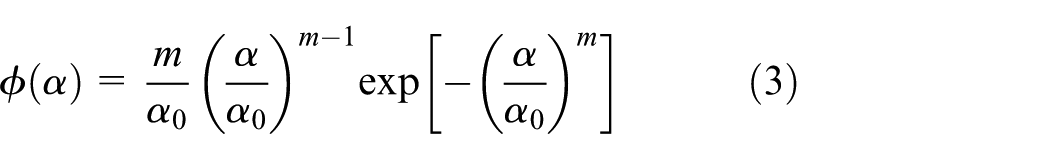
where the parameter m reflects the degree of heterogeneity of the material. The larger the value of m is, the more homogeneous the material is. Herein, the value of m is taken as 1.5. For details about the parameter selection, please refer to Zhang and colleagues;^3,22α is a certain material mechanical parameter of elements. α₀ is the average values of material properties. The computational material parameters listed above are the average values of rock properties.

In order to simulate the friction effect between the sample and the loading plate, two load pads of 10 mm × 100 mm were added on both ends of the specimen. In the meanwhile, this processing can eliminate the end effect of uneven force caused by the destruction of the boundary elements. The elastic modulus of load pads is 10 times while the uniaxial compression strength is 20 times as that of rock specimens. The whole loading process of the rock is controlled by a gradually increased compressive displacement with an increment of 0.001 mm/step.

Simulation results of rock failure process

The simulation results of rock failure process under uniaxial compression are shown in Figure 1. The shear stress field in the rock specimen is placed in the upper row. The brightness represents the size of shear stress. The distribution of failed elements is put in the lower row. Larger circles indicate the greater is the energy released by failed elements. The relationship curve of failed element events at each loading step is shown in Figure 2.

Figure 1.

Rock uniaxial compression failure process.

Figure 2.

The relationship between the element failure events and loading step.

From Figures 1 and 2, we can see that the whole loading process in rock can be divided into four stages. (1) Elastic deformation to stable microcracking development stage (section OA). (2) Yield deformation stage (section AB). Point A is the yield point, at the 52nd loading step. The element damage distribution is still random, scattered when the rock specimen just enters into the yield deformation stage at the Step 72-3. When the outer load is near peak strength, rock failure shows weak self-organization. (3) Strain softening stage (section BC). After the peak load, due to the rapid microfracturing localization, a small stress drop was generated, as shown in Step 82-23. At this stage, the element destruction is no longer in random and independent distribution; there is a synergistic interaction between adjacent elements, even in the micro elements of the entire rock system. In this way, the microcracks self-organized from disorder to orderly evolution, from random, scattered distribution to the cluster along the final rupture surface. Therefore, it is beneficial for understanding the producing mechanisms behind the following statistical microfracturing laws. (4) Residual deformation stage after ultimate unstable failure (the section after the point D). Rock blocks produced after unstable failure would slip along the macroscopic rupture surface.

Statistical analysis of the evolution of microcracks

In the RFPA^2D code, the research model studied is evenly divided into small squares of equal size, each of which is a single basic element. When two adjoining elements sharing at least one side are destructive, it is defined that they belong to the same damaged element group. Therefore, the damaged elements in a diagonal line do not be considered in the same damage group. In order to better explain the meaning of the damage group, Figure 3 gives a simple example. Figure 3 shows a numerical model and shear stress distribution at a certain loading step. In Figure 3(a), the brightness of the element represents the size of the elastic modulus. The greater the elastic modulus is, the brighter the element appears. From Figure 3(a), we can see that the brightness of the elements varies, which means that the composition of the material is heterogeneous. In Figure 3(b), the greater the shear stress is, the brighter the element shows. If the stress state of the element meets the failure criterion (a revised Coulomb’s criterion), RFPA^2D then treats the element by reducing its elastic modulus and strength. The black elements encircled by a box in Figure 3(b) are grouped together, which denotes a damaged element group. The other black elements in Figure 3(b) are a single damaged element, without forming a damage group. By this means, the length of each broken square is equal to the size of the element. The size of each damaged element group is determined by the number of elements occupied by the same damaged group.

Figure 3.

One simple example: (a) numerical model and (b) sketch map of damaged element group.

In practical experiments, the failed element group represents the microcracks in rock, and the number of the damage group indicates the number of microcracks. Here, we use S = 1, 2, 3,… to denote the size of the damaged element group. N(S) represents the number of damage group in the size S. Table 1 lists the sizes of the damaged element groups and their corresponding numbers generated by some key steps corresponding to Figure 1 in the whole failure process.

Table 1.

Damage group sizes and corresponding numbers in the whole failure process.

Step
72		81		82		97		98		150
S	N(S)	S	N(S)	S	N(S)	S	N(S)	S	N(S)	S	N(S)
1	338	1	391	1	397	1	438	1	419	1	423
2	43	2	66	2	80	2	91	2	93	2	99
3	9	3	19	3	25	3	27	3	31	3	30
4	6	4	12	4	20	4	27	4	21	4	23
5	4	5	6	5	9	5	13	5	9	5	9
6	1	6	3	6	5	6	6	6	7	6	6
		7	2	7	2	7	11	7	9	7	9
		9	2	8	3	8	3	8	3	8	2
		10	1	9	3	9	6	9	4	9	4
				10	3	10	3	10	1	11	1
				11	3	11	7	11	3	12	3
				12	2	12	4	12	5	13	2
				22	1	16	1	13	1	16	2
						17	2	16	2	17	1
						19	2	17	2	18	1
						22	1	18	1	20	2
						24	2	19	1	21	1
						46	1	20	2	27	1
						50	1	24	2	28	1
						80	1	27	1	30	1
								32	2	37	1
								35	1	51	1
								37	1	67	1
								38	1	77	1
								50	1	78	1
								63	1	88	1
								77	1	94	1
								88	1	123	1

The negative power law distribution of damaged element groups

According to the theory of SOC, when the system is approaching a SOC state, even a slightest external disturbance may cause a series of avalanche-like chain reactions.^7,8 The avalanche-like occurrences are composed of few major ones and many minor ones. The sizes of certain occurrences had a negative power relation with their frequencies. Therefore, the frequency (denoted as N) of the occurrence in size A can be shown as follows

N \propto A^{- α}

(4)

where N is the frequency, A stands for the size, and α is a constant. The relation between the frequency and the size complies with a negative power law. In other words, major occurrences are associated with low frequency while minor ones are associated with high frequency.

The size of damaged element groups (denoted as S) is equivalent to A in equation (4); the number of damaged element groups (denoted as N) is equivalent to N in equation (4). Figure 4 shows the regression fitting curve of power exponent by least squares methods, corresponding to the loading steps in Table 1.

Figure 4.

The relationship between damage group size and corresponding counts.

From Figure 4, it can be seen that the power exponents in the formula of power function vary in different stress stages of the whole failure process. Thus, it can be concluded that the microcrack distribution in the whole failure process accords with negative power laws, showing fractal features of a self-similarity structure.^23,24 When approaching a SOC state, the power exponent does not vary drastically, remaining around 1.5 approximately. The power exponent decreases correspondingly as the stress increases. This is consistent with the findings in the seismology²⁵ that the probable value of α ranges around 1.5 approximately. The minimum correlation coefficient R is 0.8633, showing a pretty high fitting relativity in the entire fitting process.

The self-similarity structure of spatial domain

The self-similarity system means that a certain structure or process appears to be self-similar even in different spatial or temporal scales, or that the local property or structure is similar with the overall property or integral structure. In addition, self-similarity also exists between the entirety or between the parts.^23,24 In terms of self-similarity, if one part of the figure is to be amplified, its structure is identical to the entirety (or the main) structure. If the structure is completely identical to the overall structure, it is called complete self-similarity; if the structure is identical to the main structure, it is called self-similarity in statistical sense.²⁶

Self-similarity can be interpreted as follows: the self-similarity structure remains unchanged when the scale r is substituted by λr. In essence, the structure is merely the amplification or contraction on the basis of its original structure. λ is named as “scale factor.” The invariance of scale transformation is called as “scale invariance.”

It can be deduced from the above distribution of negative power law between the frequency and the size, the size and its numbers of damaged element groups satisfy the negative power law function, which is shown as follows

D (V) = K V^{- α}

(5)

If the V in equation (5) is substituted by λV, the formula can be transformed to

D (λ V) = K {(λ V)}^{- α}

D (λ V) = K λ^{- α} V^{- α} = λ^{- α} K V^{- α} = \frac{1}{λ^{α}} D (V)

From the above transformation, it can be observed that the distribution curve of negative power law function remains basically unchanged when the scale changes. The distribution curve is just the amplification or contraction on the basis of the original one. Therefore, it can be regarded as a self-similarity structure.

In this numerical test, the damaged element group (microcracks) produced in the rock failure process satisfies with the distribution of negative power laws. It is a kind of self-similarity in statistical sense, not a complete one. It can be deduced that the microcracks produced in the rock failure process are always showing self-similarity features. However, it is also found from this numerical test that the value of α varies in different stress stages. When approaching the critical point of self-organization, the self-similarity structure is the most noticeable, with the value of α ranging around 1.5.

The scale invariance and long-range correlations in temporal domain

In RFPA^2D, when an element gets damaged, the elastic energy stored in the element will be released in AE according to the reduction of material parameters. The distribution of AE sequence (or failed element events) is shown in Figure 5, which displays clearly the relationship between AE frequency and time steps.

Figure 5.

The relationship between AE frequency (failed element counts) and time step.

Through analyzing the frequency curve of AE shown in Figure 5, it can be seen that the overall AE frequency at monitoring intervals is composed of few major AEs and many minor ones. During the elastic deformation phase, there is no AE recorded; when the rock samples begin to enter the yield deformation phase, the failed elements produced are still quite rare; but as the yield deformation increases gradually, the failed elements increase correspondingly; when reaching the peak strength, there is one large-scale AE event; and then as the stress declines gradually, the samples enter the strain-softening phase; when reaching the long-term strength of the rock sample, macro-rupture occurs, causing the sharp decline of stress and massive AEs. What follows is the analysis of AE sequences recorded in terms of scale invariance and long-range correlations.

The scale invariance in temporal domain analyzed by range/standard deviation method

The scale invariance in temporal domain means that the features of temporal sequences remain unchanged as the scale of time changes. It can be analyzed by means of range/standard deviation (R/S) method. The R/S method, as a statistical method to analyze the random time series, is derived from self-affine fractal, which was put forward by British hydrographer Hurst when he studied the possibility of building reservoirs along the Nile River.²⁷ This method studies the variation features of statistical rules of time serie by changing the temporal scales. When analyzing the time series abstracted from various natural phenomena, the long-range correlations between the occurrences are usually ignored based on the assumption that the occurrences only have “memories” in the short ranges. However, the R/S empirical formula proves the long-range correlations among the occurrences. The occurrence of the subsequent events is to be influenced by the previous events. In other words, time series possess similar statistical features in different temporal scales, displaying the characteristics of long-range correlations. The R/S empirical formula reflects the scale invariance of the statistical features of time series. Even if the temporal scale is adjusted, the distribution of time series remains unchanged. Consequently, through changing the temporal scales, the rules of small temporal scales can be applied to the large temporal scales, or vice versa, offering a new perspective to approach the possible fluctuation under different scales.²⁸

Some key variables of R/S method are introduced here. Set a random time variable $ξ (t)$ , and then the mean of this variable $< ξ >_{τ}$ during time interval τ can be shown as follows

< ξ >_{τ} = \frac{1}{τ} Σ_{t = 1}^{τ} ξ (t)

(6)

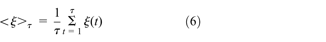
The accumulated deviation X(t, τ) can be defined as

X (t, τ) = Σ_{u = 1}^{t} (ξ (u) - < ξ >_{τ}) (t = 1, 2, 3, \dots, τ)

(7)

The range $R (τ)$ between the maximum value and the minimum value of the accumulated deviation $X (t, τ)$ is

R (τ) = \max_{1 \leq t \leq τ} X (t, τ) - \min_{1 \leq t \leq τ} X (t, τ)

(8)

The standard deviation S can be defined as

S (τ) = {[\frac{1}{τ} \sum_{t = 1}^{τ} {(ξ (t) - {〈 ξ 〉}_{τ})}^{2}]}^{1 / 2}

(9)

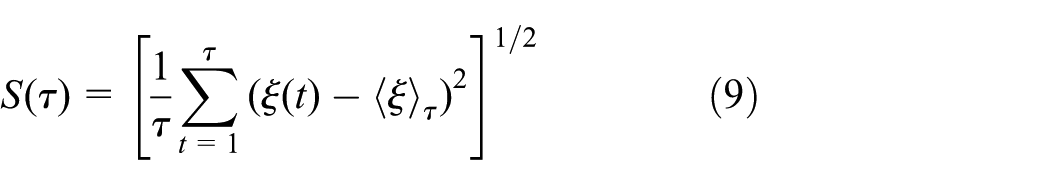
The dimensionless value of R/S in different time intervals τ satisfies the following empirical formula

\frac{R (τ)}{S (τ)} ~ τ^{H}

(10)

Equation (10) is called R/S empirical formula, in which H denotes Hurst exponent. Correspondingly, this statistical method is called R/S method. According to the above procedures, the normalization range (R/S) values of 22 loading (time) steps were analyzed respectively. Figure 6 displays the corresponding relation curve of R/S values and 22 time steps. Figure 7 presents the regression fitting curve of the logarithms of R/S value and time step (T) (Log₁₀(R/S) – Log₁₀ T) from the 98th step to 150th step. From Figure 7, it can be observed that the AEs after the 98th step obey a certain rule that the Log₁₀(R/S) regression value fits a sloping line. This indicates that there is a power relation between the R/S and time scales, $R (τ) / S (τ) ~ τ^{H}$ for AE sequences and the Hurst exponent is 0.9312, far above 0.5. Meanwhile, it also indicates that the AE sequences possess temporal scale invariance when the sample reaches the self-organization criticality state.

Figure 6.

The relation curve of R/S values and 22 time steps for the AE time series.

Figure 7.

The regression fitting curve of the logarithms of R/S value and time step (T) from step 98 to step 150.

Figure 8 presents the standard deviations of the 22 time steps, from which the dispersion of the AE frequency from the mean value of the entire AE sequence at each time step can be obtained. From Figure 8, it can be observed that when the sample is approaching the self-organization criticality state, the dispersion degree of its AE frequency from the mean value increases dramatically until the rock sample enters a self-organization criticality state.

Figure 8.

The standard deviation of AE time sequence under different research scales.

The relationship between Hurst exponent (H) and fractal dimension (D) can be shown as follows

D = 2 - H

(11)

The R/S method has a close relationship with fractal, which makes itself to be one of the key methods to estimate the fractal dimension of time series.^29–31 In this numerical simulation, at the 98th time step in a SOC state, the fractal dimension value is 1.2503 and the Hurst exponent value is 0.9312, which roughly satisfies the above formula.

The long-range correlations in temporal domain analyzed by correlation function method

In general, the long-range correlation refers to the fact that the past events still exert some influence on the subsequent events and this influence would exist even after a comparatively long time delay. The long-range correlation can be measured with the correlation function between two temporal points.³² To a physical variable x(t), its correlation function can be defined as c_x(τ) = [x(t), x(t+τ)]. If c_x(τ) declines more slowly than the exponential function, or the correlation between two points does not decline to zero in the long time range, it can be deduced that there exists long-range correlation in this system.

To a classical balanced system with random fluctuation, we can set x to denote the fluctuation variable. Then A(x) stands for the value of each measurement, the mean of which can be shown as $〈 A (x) 〉$ . The fluctuation δA(x) can be presented as

δ A (x) A (x) - 〈 A (x) 〉

(12)

The correlation function under k time delay is as follows

ρ (x) = \int_{- \infty}^{+ \infty} δ A (x_{i}) δ A (x_{i + k}) d x_{i}

(13)

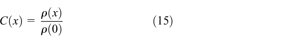
Given that the measuring points A(x) are limited, the integration ρ(x) can be substituted by the average of the sum of $δ A (x_{i}) δ A (x_{i + k})$ . Therefore, we can obtain

ρ (x) = \frac{1}{N} \sum_{x_{i} = x_{1}}^{x_{n - k}} δ A (x_{i}) δ A (x_{i + k}) = 〈 δ A (x_{i}) δ A (x_{i + k}) 〉

(14)

The correlation function ρ(x) does not rely on the measuring points A(x_i). Instead, it displays a great dependence on the intervals between measuring points (k = x_i – x_j) and the total number of measuring points (N). The self-correlation function after normalization can be shown as follows

C (x) = \frac{ρ (x)}{ρ (0)}

(15)

With the above self-correlation function, we can examine whether there exists any long-range correlation in the above-mentioned AE sequence. Set the measuring point A(x₁) as the starting point, and k = x_i – x_j = 5, 10, 15, 20, 25, 30, 35, 40, 45, 50, 55, 60, 65, 70 to 75 as the measuring intervals. Then the self-correlation of the 150 measuring points in the 150 time series (as numbered 1, 2, 3,…, 150, respectively) can be examined.

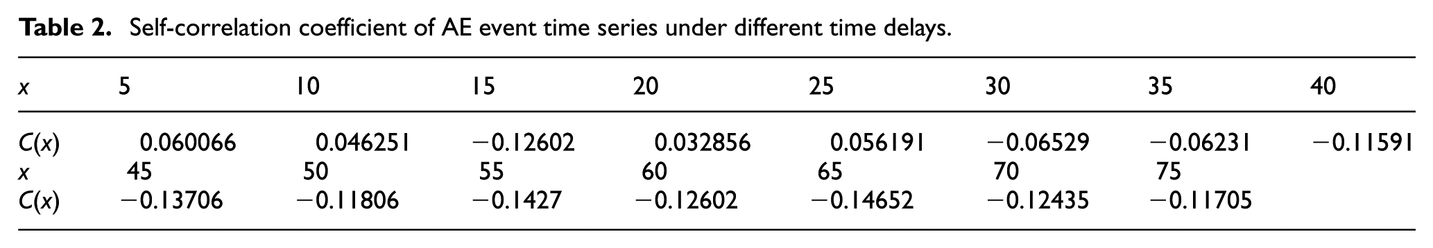
Following the above procedures, we can obtain the self-correlation coefficient under different time delays ranging from 5, 10, 15, 20, 25, 30, 35, 40, 45, 50, 55, 60, 65, 70 to 75 in turn, which is shown in Table 2. The corresponding absolute value of self-correlation coefficient is shown in Figure 9.

Table 2.

Self-correlation coefficient of AE event time series under different time delays.

x	5	10	15	20	25	30	35	40
C(x)	0.060066	0.046251	−0.12602	0.032856	0.056191	−0.06529	−0.06231	−0.11591
x	45	50	55	60	65	70	75
C(x)	−0.13706	−0.11806	−0.1427	−0.12602	−0.14652	−0.12435	−0.11705

Figure 9.

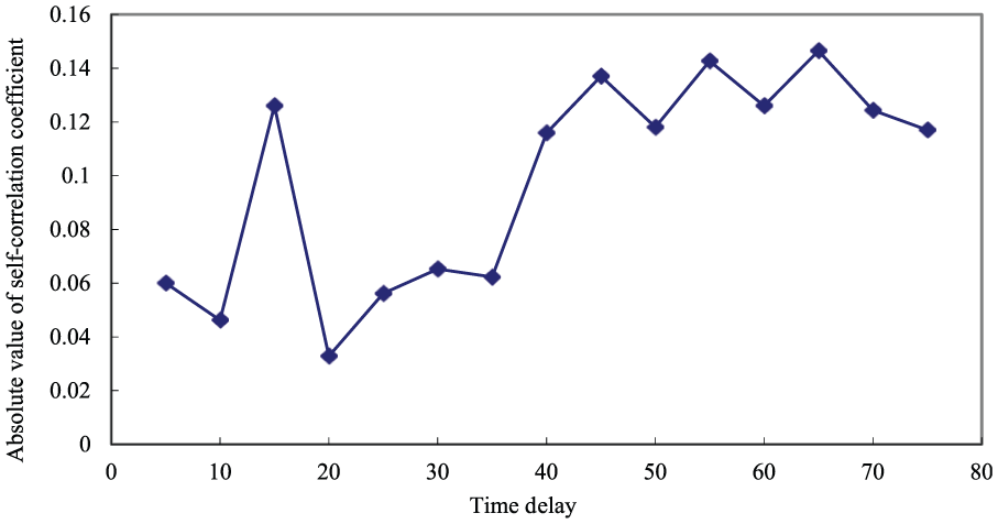
Absolute value of self-correlation coefficient of AE series with different time delays.

As can be seen from Figure 9, the absolute value of the self-correlation coefficient of AE sequence demonstrates a subsequent precursory increase (not approaching to zero) after a long time delay (e.g. 75 time steps delay).²⁵ This indicates a strong long-range correlation in AE event time series.³³

Conclusion and remarks

The microfracturing (failed element) events in the whole failure process accord with negative power law distribution, showing fractal features. When approaching a SOC state, the power exponent does not vary drastically, which ranges around 1.5 approximately. The power exponent decreases correspondingly as the stress increases.

Through the rescaled range (R/S) analysis, the time series of microfracturing events exhibits the self-similar scale-invariant properties. Through the correlation function analysis, the absolute value of the self-correlation coefficient of microfracturing sequence exhibits long-range correlation characteristics. These fractal configuration and long-range correlations are two fingerprints of SOC, which demonstrates the occurrence of SOC in rock failure.

Some information before rock unstable failure appears, for example, the decrease of the power exponent, the R/S values and the violent increases of the S value. These phenomena can be thought as some premonition and forewarning information for the coming occurrence of rock unstable failure. However, the critical point for the predicting the unstable failure is difficult to be ascertained.

Footnotes

Acknowledgements

The authors thank the anonymous reviewers for their comments, which have significantly helped to improve this article.

Handling Editor: Zedong Wu

Declaration of conflicting interests

The author(s) declared no potential conflicts of interest with respect to the research, authorship, and/or publication of this article.

Funding

The author(s) disclosed receipt of the following financial support for the research, authorship, and/or publication of this article: This work was supported by the Fundamental Research Funds for the Central Universities (no. 2015XKZ D06).

References

Bak

Tang

Wiesenfield

Self-organized criticality: an explanation of 1/f noise. Phys Rev Lett 1987; 59(4): 381–384.

Guido

Francesco

DDT

Albert

Self-organization and annealed disorder in a fracturing process. Phys Rev Lett 1996; 77(12): 2503–2506.

Zhang

Zhao

Tang

et al . Numerical study of shear behavior of intermittent rock joints with different geometrical parameters. Int J Rock Mech Min Sci 2006; 43(5): 802–816.

Lebedev

Ostrovskii

Sutin

AM.

Nonlinear acoustic spectroscopy of local defects in geomaterials. Acoust Phys 2005; 51(S1): 88–101.

Modiriasari

Bobet

Pyrak-Nolte

LJ.

Active seismic monitoring of crack initiation, propagation, and coalescence in rock. Rock Mech Rock Eng 2017; 50: 2311–2325.

Zhang

Tannant

Jing

et al . Evolution of cohesion and friction angle during microfracture accumulation in rock. Nat Hazards 2015; 77(1): 497–510.

Zhang

Tang

et al . A new numerical approach for studying self-organized criticality behavior in rock failure process. In: Liu

Tan

VBC

Han

(eds) Computational methods. Berlin: Springer, 2006, pp.1841–1846.

Yin

Dai

Wang

et al . Characteristics of bifurcation, chaos and self-organization of evolution of micro-cracks in rock. Chin J Rock Mech Eng 2002; 21(5): 635–639.

Xie

Chen

ZD.

Fractal geometry and fracture of rock. Acta Mech Sinica 1988; 4(3): 255–264.

10.

Sammis

King

GCP

. Mechanical origin of power law scaling in fault zone rock. Geophys Res Lett 2007; 34(4): L04312.

11.

Liang

et al . Mechanical and acoustic emission (AE) characteristics of rock: effect of loading and unloading confining pressure at the postpeak stage. J Nat Gas Sci Eng 2017; 44: 54–64.

12.

Gong

Chang

Three-dimensional characterization of multi-scale structures of the Silurian Longmaxi shale using focused ion beam-scanning electron microscopy and reconstruction technology. J Nat Gas Sci Eng 2017; 46: 26–37.

13.

Zhao

Zhu

Dong

YH.

Comparison of low-field NMR and microfocus X-ray computed tomography in fractal characterization of pores in artificial cores. Fuel 2017; 210: 217–226.

14.

Zhao

Jiang

YD.

Acoustic emission and thermal infrared precursors associated with bump-prone coal failure. Int J Coal Geol 2010; 83(1): 11–20.

15.

Zhang

Nunoo

Tannant

et al . Numerical study of the evolution of cohesion and internal friction in rock during the pre-peak deformation process. Arab J Geosci 2015; 8(6): 3501–3513.

16.

Tang

CA.

Numerical simulation of progressive rock failure and associated seismicity. Int J Rock Mech Min Sci 1997; 34: 249–262.

17.

Weibull

A statistical distribution functions of wide applicability. J Appl Mech 1951; 18: 293–297.

18.

Hudson

Fairhurst

Tensile strength, Weibull’s theory and a general statistical approach to rock failure. In: Proceedings of the civil engineering materials conference, Southampton, 1969, pp.901–904. London: John Wiley & Sons.

19.

Brady

BHG

Brown

. Rock mechanics for underground mining. 2nd ed. London: Chapman & Hall Press, 1993.

20.

Zhu

Tang

CA.

Micromechanical model for simulating the fracture process of rock. Rock Mech Rock Eng 2004; 37(1): 25–56.

21.

Zhang

Tang

et al . Discussion on self-organized criticality in rock failure progress. Northwest Seismol J 2006; 28(1): 1–5.

22.

Song

Zhang

Liang

et al . Effect of element size on rock shear strength and failure pattern by finite element analysis. Key Eng Mater 2005; 297–300: 2573–2578.

23.

Xie

HP.

Introduction to fractal and rock mechanics. Beijing, China: Scientific Press, 1996, pp.29–158.

24.

Zhang

JZ.

Fractal. Beijing, China: Tsinghua University Press, 1995, pp.1–18.

25.

Lei

Satoh

TS.

Indicators of critical point behavior prior to rock failure inferred from pre-failure damage. Tectonophysics 2007; 431(1): 97–111.

26.

Sornette

Power laws without parameter tuning: an alternative to self-organized criticality. Phys Rev Lett 1994; 72(14): 2306–23011.

27.

Hurst

Black

Simaike

YM.

Long-term storage: an experimental study. London: Constable, 1965.

28.

Chen

Rescaled range (R/S) analysis on seismic activity parameters. Acta Seismol Sin 2001; 23(2): 143–150.

29.

Boschette

Dentith

List

RD.

A fractal-based algorithm for detecting first arrivals on seismic traces. Geophys 1996; 61(4): 10952–11102.

30.

Dolan

Bean

CJ.

Some remarks on the estimation of fractal scaling parameters-from borehole wire-line logs. Geophys Res Lett 1997; 24(10): 1271–1274.

31.

Goltz

Fractal and chaotic properties of earthquakes. Berlin: Springer-Verlag, 1997, pp.49–55.

32.

Tian

Wang

et al . Application of correlation function in the fluctuation of excitation functions in dissipative nuclear reaction. High Energ Phys Nuc 2000; 24(2): 113–118.

33.

Yao

Jiang

LW.

Internal and external causes of working on self-organized criticality of sand piles. B Sci Technol 2003; 19(4): 278–281.

Numerical statistical analysis on self-organizing behavior of microfracturing events in rock failure

Abstract

Keywords

Introduction

Brief introduction of RFPA2D and simulated mechanism of SOC

Numerical simulation of rock failure process

Model setup

Simulation results of rock failure process

Statistical analysis of the evolution of microcracks

The negative power law distribution of damaged element groups

The self-similarity structure of spatial domain

The scale invariance and long-range correlations in temporal domain

The scale invariance in temporal domain analyzed by range/standard deviation method

The long-range correlations in temporal domain analyzed by correlation function method

Conclusion and remarks

Footnotes

Acknowledgements

Declaration of conflicting interests

Funding

References

Brief introduction of RFPA^2D and simulated mechanism of SOC