Sage Journals: Discover world-class research

Abstract

In the design and condition assessment of bridges, the extreme vehicle load effects are necessary to be taken into consideration, which may occur during the service period of bridges. In order to obtain an accurate extrapolation of the extreme value based on limited duration, threshold selection is a critical step in the peak-over-threshold method. Overly high threshold results in little information to be used and excessively low threshold leads to large bias in parameters estimation of generalized Pareto distribution. To investigate this issue, 417 days of strain data acquired from the long-term structural health monitoring system of Taiping Lake Bridge in China are employed in this article. According to the tail distribution of the strain data induced by vehicle loads, four homothetic distributions are chosen as its parent distribution, from which lots of random samples are generated by the Monte Carlo method. For each parent distribution, the 100-yearly extreme values at different thresholds are estimated and compared with the theoretical value based on those samples. Then a simple and empirical threshold selection method is proposed and applied to estimate the weekly extreme strain due to vehicle loads on the Taiping Lake Bridge. Results show that the estimate on the basis of the threshold obtained by the proposed method is closer to the measured result than the commonly used methods. The proposed method can be an effective threshold selection tool for the extreme value estimation of vehicle load effect in future engineering practice.

Keywords

Bridge health monitoring extreme value estimation generalized Pareto distribution peak-over-threshold threshold selection

Introduction

Safety assessment of bridges plays an important role in bridge management, for which the load-carrying capacity of bridges and the associated uncertainties are needed to be evaluated accurately. A large volume of research work has been conducted on the assessment of load-carrying capacity of bridges and it is possible to evaluate the load-carrying capacity reasonably.^1,2 Vehicle load effect of bridges, one of the great sources of uncertainty, is mainly studied in this article. Vehicle load effect mainly refers to stress/strain, internal force (such as bending moments, shear force), and deformation induced by vehicles passing through bridges. Obviously, vehicle load effect due to light vehicle loads is not in our concern. On the contrary, the extreme events caused by heavy vehicles, several vehicles meeting and overtaking, which endanger the serviceability and safety of bridges, are of greatest interest.

Extreme value (EV) theory indicates that EV estimation is only related to the tail of the probabilistic distribution.^3,4 Techniques and models have been developed to describe these tails, by which the probabilities of extreme events can be estimated on the basis of historical data. Among them, the peak-over-threshold (POT) method is one of the most widely used methods. It avoids the problem of wasting data, which is a common problem of the block maxima method, using a generalized Pareto distribution (GPD).⁵ However, how to select an appropriate threshold is also an inevitable problem, on which the EV estimation depends. If the threshold is too low, the tail satisfies the convergence criterion less, which will result in large bias and incorrect result. On the other hand, if the threshold is too high, little data above the threshold will lead to high variance and unreliable result.^6,7 Thus, choosing a proper threshold implies a balance between the bias and the variance.

The current methods for threshold selection mainly consist of graphic methods and computational methods.⁸ Graphic methods mainly include mean residual life (MRL) plot, Hill plot, threshold stability plot, and so on. The MRL plot, as one of the most popular used methods, has been broadly used in EV estimation of many fields such as vehicle load effect, precipitation, climate, and finance.^9–14 In this method, the threshold is selected using the plot of the mean of exceedances versus threshold. Hill plot is suitable for long-tailed distributions, which mean the shape parameter of GPD is positive. In this method, the threshold is determined by plotting the Hill estimator for a range of value of the number of upper order statistics. Computational methods are suggested to choose the optimal threshold by minimizing bias-variance of GPD model or its shape parameter based on a bootstrap procedure. For example, Caers et al.¹⁵ presented a guide to threshold selection using the finite sample mean square error (MSE) of an estimated tail parameter as a criterion. Moreover, there are some other approaches developed to address the issue. DuMouchel¹⁶ suggested using the data above tenth percentile to estimate the EV. However, theoretical examples given in this article show that these conventional methods are not suited for the EV estimation of vehicle load effect by the POT method.

In order to investigate the threshold selection method for vehicle load effect on bridge, 417 days of strain data acquired from the structural health monitoring system installed on the Taiping Lake Bridge in China are employed in this article. The strain due to vehicle loads can be obtained by the analytical modal decomposition method.^17,18 To simulate the tail distribution of vehicle load effect, four mixed distributions are chosen as the parent distributions, from which a large number of samples are produced by the Monte Carlo method. For each parent distribution, the 100-yearly EVs are estimated at different thresholds. By Comparing the estimates at different thresholds and corresponding theoretical values, an empirical threshold selection method is proposed to study the vehicle load effect.

Threshold estimation methods

Three commonly used methods are introduced in this section, including the MRL plot, Hill plot, and minimum MSE method, which will be compared with the proposed threshold selection method in this article.

The MRL plot

Davison and Smith¹⁹ introduced MRL plot to determine the threshold using the expectation of the GPD excesses

e (u) = E (x - u | x > u) = \frac{σ_{u} + ξ u}{1 - ξ}, ξ < 1

(1)

where u denotes the threshold, ξ denotes the shape parameter, and σ_u denotes the scale parameter corresponding to threshold u. The condition of ξ < 1 is defined to guarantee the existence of the expectation. Equation (1) shows that the expectation of excesses is linear in u with gradient ξ/(1 – ξ) and intercept σ_u/(1 – ξ). For a set of samples (X₁, X₂,…, X_n), the empirical estimate of the mean of excesses can be obtained as follows

e_{n} (u) = \frac{1}{N_{u}} \sum_{i = 1}^{N_{u}} (X_{i} - u), X_{i} > u

(2)

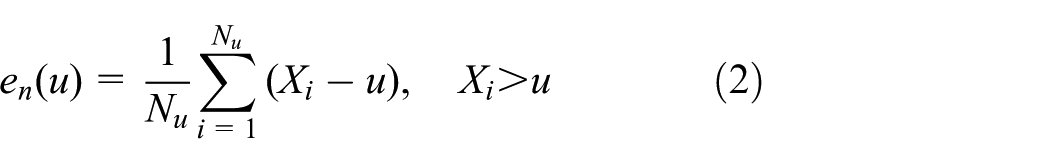
where N_u denotes the number of exceedances over u. The set data of {u, e_n(u)} represent the MRL plot. Generally, the value of u above which the plot is an approximately straight line can be selected as the optimal threshold.

Hill estimator

Let $X_{(1, n)} > X_{(2, n)} > \dots > X_{(n, n)}$ be associated descending order statistics of (X₁, X₂,…, X_n) which are independent and identically distributed random variables.²⁰ Assuming that the distribution of these random variables is heavy tailed, the Hill estimator, a well-known estimator of ξ, is defined as

H_{k, n} = \frac{1}{k} \sum_{i = 1}^{k} \log (\frac{X_{(i, n)}}{X_{(k, n)}}), k \leq n

(3)

Clearly, the Hill estimator is function of these extreme random variables {X_(1,n), X_(2,n),…, X_(k,n)} which depends on the chosen threshold. A Hill plot is constructed by the Hill estimator of a range of k values versus the k value or the threshold. The value of X_k,n above which the Hill estimator tends to be stable can be chosen as the optimal threshold.

MSE

The MSE can be evaluated on any tail characteristics θ such as the shape parameter of GPD, an extreme quantile, or a return period. The optimal threshold can be obtained by evaluating the MSE for a range of thresholds. The bootstrap is chosen as the technic to analyze estimation bias and variance of the tail characteristics θ at each threshold:

Select a range of high thresholds (u₁, u₂,…, u_j).

For each threshold $u_{i} (1 \leq i \leq j)$ :

Select the exceedances over the threshold u_i, that is, ${X_{(1, n)}, X_{(2, n)}, \dots, X_{(k_{i}, n)}}$ to fit the GPD and then evaluate the estimate ${\hat{θ}}_{i}$ .

For each bootstrap loop: draw a resample ${X_{2}^{(b)}, X_{2}^{(b)}, \dots, X_{k, n}^{(b)}}$ and then evaluate the estimate ${\hat{θ}}_{i}^{(b)}$ using the bootstrap data.

Calculate the MSE of $\hat{θ} (u_{i})$ according to the estimates.

The optimal threshold is selected when MSE of $\hat{θ} (u)$ is approaching the minimum.

Since threshold selection greatly influences the parameter estimation of a GPD, the shape parameter ξ is chosen as the tail characteristic θ in this article.

Threshold estimation based on the EV extrapolation of strain data

Simulation of strain peaks distribution induced by vehicle loads

It is demonstrated that the EV estimation corresponds to tail data.³ To ascertain the probability distribution of the tail data of vehicle load effect, the strain data of 417 days of a long cable-stayed bridge in China is taken as the real example. The strain due to vehicle loads can be obtained by decomposing the measured strain through analytical model decomposition method. Figure 1 shows the strain time history due to vehicle loads on 27 December 2015. Each “jump” in the figure represents the strain time history induced by a vehicle passing through the bridge. The maximum value of each “jump” is defined as strain peak, which is assumed to be independent.^21,22 According to the suggestion in DuMouchel,¹⁶ the upper 10% of these strain peaks, which is larger than 18.1 με, are collected. It is indicated that mixed distributions of normal distribution, lognormal distribution, and Weibull distribution can fit vehicle load and its effect well.^23–24 Since the histogram of collected data shows three peaks, three mixed distributions (a mixed distribution of three normal distributions, a mixed distribution of one lognormal and two normal distributions, a mixed distribution of one Weibull and two normal distributions) are chosen to fit these collected data, as shown in Figure 2. The Kolmogorov–Smirnov test for goodness-of-fit is used. Results show that all the three models coincide with the tail data well, and the third model, that is, a mixed distribution of one Weibull and two normal distributions, is the best. The same conclusion can be drawn from the strain peaks collected from other four measurement points on the bridge. In order to investigate the influence of threshold on EV estimation in POT method, four homothetic parent distributions are given to simulate the tail distribution of vehicle load effect as follows:

A mixed distribution of three normal distributions;

A mixed distribution of one lognormal and two normal distributions;

A mixed distribution of one Weibull and two normal distributions;

A mixed distribution of one Weibull and two normal distributions with different parameters.

Figure 1.

Strain peaks induced by vehicle loads of Taiping Lake Bridge (27 December 2015).

Figure 2.

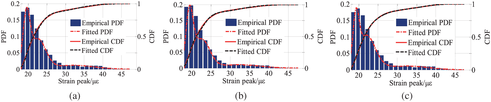
Strain peaks over 18.1 με fitted by the three mixed distributions. (a) The mixed distribution of three normal distributions—p₁ = 0.3665, µ_N₁ = 18.56, σ_N₁ = 0.94; p₂ = 0.4708, µ_N₂ = 22.62, σ_N₂ = 2.09; p₃ = 0.1627, µ_N₃ = 32.21, σ_N₃ = 5.45. (b) The mixed distribution of one lognormal distribution and two normal distributions—p₁ = 0.4055, µ_L₁ = 2.98, σ_L₁ = 0.052; p₂ = 0.4388, µ_N₂ = 22.82, σ_N₂ = 2.12; p₃ = 0.1558, µ_N₃ = 32.56, σ_N₃ = 5.38. (c) The mixed distribution of one Weibull distribution and two normal distributions—p₁ = 0.7593, µ_N₁ = 18.1, σ_W₁ = 5.62, ζ_W₁ = 0.9796; p₂ = 0.0953, µ_N₂ = 19.93, σ_N₂ = 0.71; p₃ = 0.1454, µ_N₃ = 21.98, σ_N₃ = 1.34.

Probability models of the third and fourth parent distributions are the same, while the parameters are different. Parameters of the four parent distributions are listed in Table 1.

Table 1.

Parameters of four parent distributions.

Parent distribution	p₁	p₂	p₃	The first component	The second component	The third component
1	0.6	0.25	0.15	μ_N = 26, σ_N = 0.8	μ_N = 30, σ_N = 4	μ_N = 40, σ_N = 6
2	0.75	0.15	0.1	μ_L = 3, σ_L = 0.2	μ_N = 28, σ_N = 2.5	μ_N = 35, σ_N = 5
3	0.7	0.2	0.1	σ_w = 5, ξ_w = 1.2, μ_w = 32	μ_N = 37, σ_N = 1.5	μ_N = 40, σ_N = 4
4	0.75	0.1	0.15	σ_w = 4.5, ξ_w = 1.3, μ_w = 20	μ_N = 20, σ_N = 1	μ_N = 23, σ_N = 1.5

p₁, p₂, p₃ denote the weighting coefficients; μ_N, σ_N denote the mean value and standard deviation of Normal distribution, respectively; μ_L, σ_L denote the mean value and standard deviation of Lognormal distribution, respectively; σ_w, ξ_w, μ_w denote the scale parameter, shape parameter, and position parameter of Weibull distribution, respectively.

With reference to the measured data of Taiping Lake Bridge, 100 strain peaks, which are in the top 10%, are supposed to be produced every day. From each parent distribution, 100 times for different data length (such as a day, a month, 6 months, a year, 10 years and 50 years) are randomly sampled by Monte Carlo method, which means 100 groups, respectively, with the sample size of 100, 3000, 18,000, 36,000, 360,000, and 1,800,000 are sampled from each parent distribution.

Threshold estimation of samples generated from the fourth parent, which is apparently the closest to the optimal model shown in Figure 2(c), is analyzed in detail, while the other three examples are presented in Appendix 1.

The effect of threshold chosen on EV estimation

A series of values chosen as thresholds are listed in Table 2. The mean number of exceedances over each chosen threshold is calculated and also shown in the table. The exceedances are fitted by GPD models. Parameters of GPD can be estimated by the maximum likelihood.¹⁵ The fitting residual can be obtained as follows

Fitting residual = \frac{1}{N} \sum_{i = 1}^{N} | F (x_{i, N}) - \hat{F} (x_{i, N}) |

(4)

Table 2.

The number of exceedances over different thresholds (the fourth parent distribution).

Sampling time (d)	Threshold (u)
Sampling time (d)	32	34	36	38	40
30	62.74	27.9	11.81	4.99	1.74
180	375.48	170.8	75.49	31.97	12.94
360	753.33	337.92	146.25	61.89	25.92
3600	7523.3	3408.3	1486.7	627.41	257.4
18,000	37,674	17,020	7427.8	3144	1288.6

which is used as a goodness-of-fit function for GPD. F(x_i,N) denotes the empirical cumulative probability at value of x_i,N, and $\hat{F} (x_{i, N})$ denotes the cumulative probability calculated from GPD at x_i,N. The mean values of fitting residual of 100 group samples with the same sampling length are listed in Table 3. Then, 100-yearly EV at each chosen threshold is estimated as follows

F_{M} (x) = \exp [- λ T_{p} (1 - G (x))]

(5)

Table 3.

Fitting residual of GPD model (the fourth parent distribution).

Sampling time (d)	Threshold (u)
Sampling time (d)	32	34	36	38	40
30	0.0275	0.0418	0.0698	–	–
180	0.0136	0.0181	0.0265	0.0389	0.0680
360	0.0092	0.0120	0.0177	0.0271	0.0428
3600	0.0069	0.0063	0.0071	0.0094	0.0136
18,000	0.0065	0.0057	0.0054	0.0053	0.0070

GPD: generalized Pareto distribution.

Where “–” denotes that data are too little to be used, same denotation is adopted in the following tables.

where T_p, λ, and G(x) denote the forecast period (T_p = 100), the number of exceedances per year, and fitted GPD, respectively. Characteristic value of the expectation of each 100-yealy EV distributions is calculated. The mean value, the standard deviation, and 95% confidence interval (CI) of the characteristic values are listed in Table 4. Since the fourth parent distribution is known, the theoretical characteristic value can be obtained, which is 56.82.

Table 4.

Estimates of 100-yearly EV (theoretical value E = 56.82).

Sampling time (d)		Threshold (u)
Sampling time (d)		32	34	36	38	40
30	μ, σ	63.47, 11.47	62.45, 14.37	59.75, 8.64	–	–
	95% CI	[54.22, 78.86]	[51.79, 83.13]	[47.21, 73.95]	–	–
180	μ, σ	61.75, 5.52	60.70, 4.89	60.56, 6.24	59.94, 6.44	57.98, 4.60
	95% CI	[58.47, 68.56]	[55.32, 67.67]	[54.65, 71.40]	[51.14, 69.30]	[49.55, 67.07]
360	μ, σ	60.98, 4.39	60.66, 4.58	60.47, 5.27	59.60, 4.61	58.74, 4.32
	95% CI	[58.45, 63.31]	[57.16, 66.50]	[55.83, 66.46]	[53.52, 67.96]	[52.48, 64.94]
3600	μ, σ	60.97, 4.16	59.96, 3.17	59.26, 2.52	58.89, 2.48	58.86, 3.07
	95% CI	[60.16, 61.61]	[59.00, 60.79]	[57.88, 60.39]	[57.36, 62.15]	[56.53, 63.86]
18,000	μ, σ	60.94, 4.12	59.98, 3.17	59.24, 2.43	58.67, 1.92	58.33, 1.72
	95% CI	[60.74, 61.17]	[59.62, 60.37]	[58.68, 59.78]	[57.80, 60.12]	[57.17, 60.35]

EV: extreme value; CI: confidence interval.

Where μ, σ denote the mean value and standard deviation of characteristic values, respectively; same denotations are adopted in following tables.

From Table 4, it can be found that estimates of EV depend on the threshold and sample size. Obviously, larger sample size will bring better estimates, while choosing an appropriate threshold involves a trade-off between the bias and the variance. In order to select the optimal threshold, the MSE criterion is applied as

MSE = bia s^{2} (E - μ) + σ^{2}

(6)

where μ, E, and σ² denote the mean value, the theoretical value, and the variance of characteristic value, respectively. The threshold achieves optimal when MSE reaches the minimum. Moreover, it is assumed that relative error less than 10% is within acceptance range. For the fourth parent distribution, the 95% CI of characteristic value in the interval [51.14, 62.50] is allowed.

Analyzing Tables 2 –4, some conclusions can be drawn as follows: the estimate of EV based on a GPD is larger than the theoretical value generally. It is not advisable to estimate the EV based on 1 day’s data. Satisfied results cannot be obtained based on data of 1 month or 6 months or 1 year either, since 95% CI of the characteristic value exceeds the acceptable range. In all of the above cases, better estimate can be achieved with a larger threshold. Based on 10 years’ data, satisfied results can be obtained when the threshold is in the interval [34, 38], and the best estimate is achieved with the threshold of 38. When the sampling time is as long as 50 years and the threshold is within the interval [34, 40], the estimates are good which achieve the best with the threshold of 40. Moreover, better results of estimate cannot be guaranteed by better fitting results of GPD model. The variation of estimates with threshold of samples produced from the other three parent distributions is similar to that of the fourth.

Threshold estimation

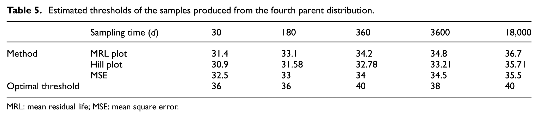
For each group of samples, the thresholds are estimated by the MRL plot, Hill plot, and MSE method. The mean values of thresholds of the samples with the same sampling length and the optimal threshold are listed in Table 5.

Table 5.

Estimated thresholds of the samples produced from the fourth parent distribution.

	Sampling time (d)	30	180	360	3600	18,000
Method	MRL plot	31.4	33.1	34.2	34.8	36.7
	Hill plot	30.9	31.58	32.78	33.21	35.71
	MSE	32.5	33	34	34.5	35.5
Optimal threshold		36	36	40	38	40

MRL: mean residual life; MSE: mean square error.

As shown in Table 5, thresholds estimated by the three methods increase with the increasing of sample size. It can also be found that the thresholds estimated by the three methods are smaller than the optimal thresholds generally. Similarly, the threshold estimation results of the other three parent distributions also are not very good, which mean that the commonly used methods are not suitable for investigating the vehicle load effect. In addition, a significant drawback of the graphic methods is that the MRL plots and Hill plots of samples generated from the same parent distribution show great instability. Especially, for the third and fourth parent distribution, more than 80% of the MRL plots and Hill plots are difficult to determine the “turning point,” that is, the threshold.

Based on the estimated EV at different thresholds of four parent distributions, an empirical threshold estimation technic based on the relationship between the characteristic value and the threshold is proposed in this article. The steps are as follows: draw the plot of characteristic value versus the threshold and observe the relationship between them. (1) If the sample size is large enough, the characteristic value tends to be stable with the increasing of threshold. In this case, the starting point of stable region can be selected as the optimal threshold. (2) If the sample size is small, the variation magnitude of characteristic value remains constant or even increases with the increasing of threshold, and it does not tend to be stable. In this case, the threshold should be as large as possible under the condition that shape parameter of GPD can be correctly estimated without large fluctuations or obvious errors.

Case study—Taiping Lake Bridge

The Taiping Lake Bridge is a pre-stressed concrete cable-stayed bridge with single cable plane and single tower, locating in Huang Mountain scenic spot of Anhui Province in China.²⁵ The bridge has a length of 380 m (span combination: 190 m + 190 m), as shown in Figure 3. The bridge carries four lanes with a width of 14 m. The health monitoring system was installed on the bridge in 2014 to collect information for bridge safety assessment. Measurement points are selected at several locations of the box girder. Strain gauges are installed at bottom plate of the main girder with a sampling frequency of 50 Hz. These strain gauges are arranged along the longitudinal direction of the bridge. By comparing the strain of different measuring points, the strain data of the most dangerous section under vehicle loads is studied which locate at about 121 m from the centerline of tower.

Figure 3.

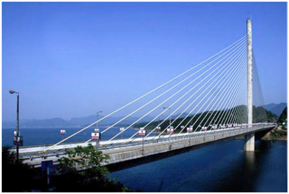
The Taiping Lake Bridge (Huang Mountain, China).

Taking 417 days’ strain data (2015.4–2016.7) of the bridge as the real example, all strain peaks induced by vehicle loads are extracted as samples. Several thresholds are selected, and then the corresponding 100-yearly EV distributions are estimated based on GPD. The plot of expectation of the EV versus threshold is shown in Figure 4. From this figure, it can be seen that when the threshold is greater than 41, the expectation varies slowly. Thus, it is suggested to choose 41 as the optimal threshold. To evaluate the optimal threshold, the measured data of 417 days is divided into two parts, while data of the first 67 days are used to estimate weekly EV, and the remaining data of 350 days, that is, 50 weeks, are used to validate the estimate. The estimated and measured weekly EV distributions are shown in Figure 5. It can be found that the estimate coincides with the measured result well. However, the EV estimated by GPD is a little bit larger than measured value. Moreover, the MRL plot and Hill plot of these strain peaks are shown in Figure 6, and the thresholds estimated by the three common methods are listed in Table 6. The weekly extreme strain distribution at each threshold is estimated. Corresponding expectations are also shown in table, which indicates that the estimate by the proposed technic is better than the common methods.

Figure 4.

Expectation of 100-yearly EV versus the threshold.

Figure 5.

Estimated and measured weekly extreme strain distribution.

Figure 6.

Threshold estimation of graphic methods: (a) MRL plot and (b) Hill plot.

Table 6.

Threshold estimated by the common methods (mean of measured weekly extreme strain: 40.89 με).

Method	MRL plot	Hill plot	MSE method	The proposed method
Estimated threshold (με)	39.06	39.57	39.97	41
Expectation of weekly extreme strain (με)	43.44	42.94	42.55	41.9

MRL: mean residual life; MSE: mean square error.

Conclusion

The present paper focuses on the threshold selection in POT method to estimate the EV of vehicle load effect on bridge. 417 days of strain data of a long cable-stayed bridge located in China are employed to study this issue. According to the tail distribution of strain data due to vehicle loads, four homothetic distributions are chosen as the parent distributions. On the basis of samples produced by Monte Carlo method from each parent distribution, characteristic values at different thresholds are estimated and compared with the corresponding theoretical value. Then an empirical method for the threshold estimation based on the relationship between the characteristic value and threshold is proposed. Finally, the proposed method is compared with the commonly used methods and verified based on the strain data due to vehicle loads on Taiping Lake Bridge. The conclusions are drawn as follows:

The distribution of strain peaks induced by vehicle loads is a multi-peak distribution, and the tail distribution can be described by a mixed distribution of one Weibull and two normal distributions.

The characteristic value mainly depends on threshold. With the increase of the threshold, the bias of characteristic value decreases first and then tends to be stable, while the variance decreases at first and then increases gradually. It means that an optimal threshold involves a trade-off between the bias and the variance.

The characteristic value is closely related to the sample size. If the bias does not tend to be stabilized with the increasing of threshold for the shortage of samples, the EV cannot be estimated accurately. In that case, the threshold should be as large as possible.

The estimated EV based on GPD is greater than the theoretical value generally.

On the basis of the estimated EV of Taiping Lake Bridge, it is demonstrated that compared with the commonly used methods, the proposed method is more suitable to estimate the threshold of vehicle load effect.

Footnotes

Appendix 1 Acknowledgements

We acknowledge the support received from the Anhui Provincial Natural Science Foundation (1708085ME101) and the China Postdoctoral Science Foundation (2015M581982).

Handling Editor: Kenneth Loh

Declaration of conflicting interests

The author(s) declared no potential conflicts of interest with respect to the research, authorship, and/or publication of this article.

Funding

The author(s) received no financial support for the research, authorship, and/or publication of this article.

References

Obrien

Schmidt

Hajializadeh

et al . A review of probabilistic methods of assessment of load effects. Struct Saf 2015; 53: 44–56.

Liu

Frangopol

Kim

. Bridge system performance assessment from structural health monitoring: case study. J Struct Eng 2009; 135(6): 733–742.

Shi

. Practical extremum statistical method. 1st ed. Tianjin, China: Tianjin Science and Technology Press, 2006, p.29.

De Haan

Ferreira

. Extreme value theory: an introduction. 1st ed. New York: Springer Science+Business Media, 2007, p.141.

Ding

Chen

. Assessment of methods for extreme value analysis of non-Gaussian wind effects with short-term time history samples. Eng Struct 2014; 80: 75–88.

Gomes

Guillou

. Extreme value theory and statistics of univariate extremes: a review. Int Stat Rev 2015; 83(2): 263–292.

Dupuis

. Exceedances over high thresholds: a guide to threshold selection. Extremes 1999; 1(3): 251–261.

Scarrott

MacDonald

. A review of extreme value threshold estimation and uncertainty quantification. REVSTAT: Stat J 2012; 10(1): 33–60.

Xia

. Extrapolation of extreme traffic on bridges based on long-term SHM data. Smart Struct Syst 2016; 17(6): 995–1015.

10.

Beguería

Angulo-Martínez

Vicente-Serrano

et al . Assessing trends in extreme precipitation events intensity and magnitude using non-stationary peaks-over-threshold analysis: a case study in northeast Spain from 1930 to 2006. Int J Climatol 2011; 31(14): 2102–2114.

11.

Naveau

Nogaj

Ammann

et al . Statistical methods for the analysis of climate extremes. C R Geosci 2005; 337(10): 1013–1022.

12.

Andreev

Tinyakov

Parahin

et al . An application of EVT, GPD and POT methods in the Russian stock market (RTS index), 17November2009, https://poseidon01.ssrn.com/delivery.php?ID=846003031121107088126030003114116121026078000043086087097005110074127127078092073088016013099125108026042119122120065082014084111029013011019082105126029000083110073002038091025076070071009084120126088085121121100126102107122125110098115089007001000099&EXT=pdf

13.

Gilli

këllezi

. An application of extreme value theory for measuring financial risk. Comput Econ 2006; 27(2–3): 207–228.

14.

Booij

Tong

. Uncertainty analysis in statistical modeling of extreme hydrological events. Stoch Env Res Risk A 2010; 24: 567–578.

15.

Caers

Beirlant

Maes

. Statistics for modeling heavy tailed distributions in geology: part I. Methodology. Math Geol 1999; 31(4): 391–410.

16.

DuMouchel

. Estimating the stable index α in order to measure tail thickness: a critique. Ann Stat 1983; 11: 1019–1031.

17.

Wang

Chen

. Analytical mode decomposition of a time series with overlapping and rapidly time-varying frequencies with Hilbert transform. Smart Mater Struct 2013; 22(9): 1–15.

18.

Kuang

KSC

Koh

. Acoustic emission source location and noise cancellation for crack detection in rail head. Smart Struct Syst 2016; 18(5): 1063–1085.

19.

Davison

Smith

. Models for exceedances over high thresholds. J Roy Stat Soc B Met 1990; 52(3): 393–442.

20.

Brilhante

Gomes

Pestana

. A simple generalisation of the Hill estimator. Comput Stat Data An 2013; 57(1): 518–535.

21.

Ruan

Zhou

Guo

. Extreme value extrapolation for bridge vehicle load effect based on synthetic vehicle flow. J Tongji Univ: Nat Sci 2012; 40(10): 1458–1462.

22.

. Structural health monitoring in mainland China: review and future trends. Struct Health Monit 2010; 9(3): 219–231.

23.

Guo

Frangopol

Chen

. Fatigue reliability assessment of steel bridge details integrating weigh-in-motion data and probabilistic finite element analysis. Comput Struct 2012; 112: 245–257.

24.

Sun

. Statistic model of vehicle loads for highway bridge. J Tongji Univ: Nat Sci 2012; 40(2): 198–204.

25.

Yan

Ren

. Circularly-symmetric complex normal ratio distribution for scalar transmissibility functions. Part II: probabilistic model and validation. Mech Syst Signal Pr 2016; 80(1): 78–98.

Threshold selection for extreme value estimation of vehicle load effect on bridges

Abstract

Keywords

Introduction

Threshold estimation methods

The MRL plot

Hill estimator

MSE

Threshold estimation based on the EV extrapolation of strain data

Simulation of strain peaks distribution induced by vehicle loads

The effect of threshold chosen on EV estimation

Threshold estimation

Case study—Taiping Lake Bridge

Conclusion

Footnotes

Appendix 1

Acknowledgements

Declaration of conflicting interests

Funding

References