Potential field method for persistent surveillance of multiple unmanned aerial vehicle sensors

Abstract

Persistent surveillance is one of the major tasks envisioned for unmanned aerial vehicles in that some regions of interest need to be continuously surveyed. This distinction from the one-time coverage/exploration does not allow a straightforward application of the most exploration techniques to address the persistent surveillance problem. This article introduces and demonstrates a method of alterable artificial potential field to control a group of unmanned aerial vehicles to stay over the region of interest. We present attractive potential field to drive the unmanned aerial vehicles to desirable areas, obstacle potential field to move away from obstacles, collision avoidance potential field to control unmanned aerial vehicles not to collide with others, and formation of potential field to make unmanned aerial vehicles gather in a group. The simulation results show that the proposed approach could generate collision-free path for unmanned aerial vehicles staying over the region of interest for a long endurance.

Introduction

The use of unmanned aerial vehicle (UAV) sensors has increased dramatically in civilian and military applications such as geological surveying, reconnaissance and tracking, border patrolling, environment data collection, ¹ and so on. UAVs have better performance in surveillance due to their characteristics of wide area coverage and insensitivity to terrain. One of the typical tasks involved in these missions is to monitor the region of interest (ROI) continuously, which is called persistent surveillance in this work. Persistent surveillance enables a faster decision cycle and supports the application of precision action to achieve desired effects. ² In recent years, the topic of multiple UAVs has developed into a major research interest for solving the problems of persistent surveillance in new and efficient ways. A key aspect of the multiple UAVs is that they are distributed and, therefore, do not rely on a central controller. Due to the fact that the loss or damage of individual UAV does not affect the performance of the system, multiple UAVs are higher reliable and more scalable than single complicated UAV. Moreover, multiple UAVs can provide multi-angle observations, which is very important in the surveillance task. Consequently, multiple UAVs are advantageous over single UAV for executing persistent surveillance task.

Persistent surveillance requires that a given ROI be covered continuously and completely by UAVs for collecting sensor data to generate actionable information, ³ such as identifications, locations and movements of potential targets and threats. To some extent, persistent surveillance is similar to the one-time coverage/exploration. There are also some similarities between them, for instance, reducing the unobserved area in the target space as much as possible and keeping in forming a team or a unit in task execution. Unlike the tasks of one-time coverage and exploration, however, persistent surveillance requires the UAVs to stay over the given ROI continuously over time in order to obtain the relative real-time understanding of the ROI. This difference makes the most one-time coverage/exploration techniques not be straightforwardly applied in solving the problem of persistent surveillance, but ideas behind one-time coverage/exploration methods can still be used in persistent surveillance.

One of the key issues for designing the strategy of persistent surveillance is to plan the flying paths of UAVs over an ROI. Path planning can be regarded as the process for automatically generating paths for UAVs according to some predefined standards. ⁴ In path planning, it is necessary to not only find a path that visit the ROI time and again for each UAV but also account for the obstacle avoidance of the paths. A collision with stationary structures or another UAV could prove to be potentially fatal and might even result in the failure of persistent surveillance mission. ⁵ Therefore, it is necessary for the UAVs to be able to avoid the collisions with obstacles or other UAVs successfully during the path planning. Furthermore, the paths in the mission of persistent surveillance should be feasible for UAVs to follow. The trajectories have to meet dynamic limits of UAVs. Specifically, the minimum turn radius constraint should be accounted for because UAVs cannot take sharp turns. The minimum turn radius specifies the sharpest turn that the UAV is capable of tracking. If the path of persistent surveillance designed by planners requires sharp turning beyond the dynamics limits of UAVs, the UAV will not be able to follow the path, which would result in undesirable behaviors.

As mentioned before, the key issues in persistent surveillance of multiple UAVs include (1) the UAVs should cover an ROI time and again, instead of being one time; (2) the UAVs should minimize the unobserved area as much as possible; (3) the paths of multiple UAVs for persistent surveillance should be flyable and maneuverable, in order to meet the kinematics constraints and the imposed dynamics of UAVs; and (4) the paths of UAVs have to be collision avoidance, including the obstacle collision avoidance and intra UAVs collision avoidance. The motivation of this article is to devise a collision-free path planning method to make the UAVs surveying an ROI in long duration with little unobserved area. Conventionally, path planning is responsible for producing a continuous motion that connects a start configuration and a desirable configuration. ⁶ Local collision-avoidance algorithm ensures that UAVs could avoid collision with unknown obstacles or other UAVs. Hence, the work in this article is based on global path-planning algorithms with local collision-avoidance features imbedded into it to provide persistent capability over the desired operational area. We want to utilize the potential field method which consists of “attractive field,” to pull the UAV toward the goal, and “repulsive fields,” to avoid collisions. Besides, in our study, it is imperative to consider the dynamic constraints of the vehicles.

The main contributions of our research work include the following: (1) we propose an alterable artificial potential field method to realize the path planning of UAVs over the ROI continuously and (2) the coupling problem of the UAV dynamics and path-planning policies has been taken into consideration. The reminder of this article is organized as follows: section “Related work” briefly highlights the related work. Section “Potential field methods” introduces the definition of the artificial potential field. Section “Aircraft dynamics” simplifies the dynamic model of UAVs for path planning in two-dimensional (2D) plane. Section “Alterable potential field method” presents the alterable potential field method for meeting requirements of persist surveillance. Section “Performance evaluations” conducts some simulation to validate and evaluate our proposed schemes, and conclusions are given in section “Conclusions and future work.”

Related work

There have been growing interests in control and coordination of UAVs to execute the task of exploration/coverage in past two decades. Many path planning approaches are proposed in addressing the related problems such as shortest path planning, map uncertainty reducing, the unobserved area reducing, the collision avoidance, and so on. Redding et al. ⁷ describe an effective algorithm of path planning to ensure simultaneous arrivals of heterogeneous UAVs in a dynamically varying environment. Howlett et al. ⁸ present a path planner for an UAV which is based on the learning real-time A* search algorithm and produce dynamically feasible paths that accomplish the sensing objectives in the shortest possible distance. Vincent and Rubin ⁹ design a cooperative search method that integrates the multiple UAVs into an advantageous formation in sweep searching for targets while minimizing the transmission of control information. Pongpunwattana and Rysdyk ¹⁰ introduce a market-based cooperative planning system for a team of autonomous vehicles in a dynamic uncertain environment, which could allocate tasks and plan paths simultaneously. Shaferman and Shima ¹¹ propose a distributed evolutionary-based stochastic search method for a team of heterogeneous UAVs to track targets in a known urban terrain. Prevost et al. ¹² present an extended Kalman filter–based algorithm that predicts the trajectory of a moving object from its measured position.

The potential field approach has been widely used as a navigation method in UAVs. In this method, an UAV is modeled as a moving agent under the influence of a potential field which is determined by the goal and the obstacles. The main advantage of this method over the other path-planning methods is its low calculation cost. Bennet and McInnes ¹³ developed a new bounded guidance law which is based on bifurcating potential field to achieve verifiable patterns of the formation of UAVs. Eun and Bang ¹⁴ present a new path finding and planning method for multiple UAVs which is based on the potential field theory. Incorporated with the optimal control theory, the additional control force is introduced into the artificial potential field method for the UAV path-planning problem. ¹⁵ Based on a virtual leader method and an extended local potential field, Paul et al. ¹⁶ present a solution for formation flight and formation reconfiguration of UAVs.

The above existing techniques of path planning cannot be applied in persistent surveillance directly, since they cannot guarantee the UAVs stay over the ROI for a long duration. There are some studies concerning the problems of persistent exploration by using multiple UAVs. Nigam ¹⁷ thoroughly reviews the persistent surveillance problem using UAVs. He shows that the persistent surveillance problem differs from exploration since it involves continuous/repeated coverage of target space. Zhang et al. ¹⁸ present a framework for persistent monitoring in a one-dimensional (1D) situation by mobile sensors. The 1D persistent monitoring can be interpreted as barrier coverage to detect the intruders who are attempting to cross an ROI. Arvelo et al. ¹⁹ design time-invariant memory-less control policies for robots that move in a finite 2D lattice and are tasked with persistent surveillance of an area. Alamdari et al. ²⁰ represent the environment as a graph with vertex weights and edge length and map the persistent monitoring problem into the problem of finding a way that minimizes the maximum weighted latency of any vertex. Michael et al. ²¹ focus on the detailing of system architecture capable of addressing the problem of persistent surveillance with a team of autonomous micro aerial vehicles (MAVs). They provide the hardware of the MAV and the algorithm methodology for autonomous operation. We have proposed a flocking algorithm to drive the MAVs flying in a coordinate formation with a capability of obstacle avoidance to achieve persistent surveillance. ²² Valenti et al. ²³ consider that the persistent surveillance problem belongs to the coordination of resources and present a health management technique for 24/7 persistent surveillance trying to keep at least one UAV in a target area. Redding et al. ²⁴ introduce an automated battery management for long-duration mission of multiple agents. Zhang et al. ²⁵ provide methods of energy conservation and energy balance for prolonging the lifetime of the group of agents in order to collect data continuously.

The most related work with our research is the Nigams’.^3,26,27 Nigam et al. provide a semi-heuristic approach to continuously search the ROI and minimize the time between visitations to each region. In their method, the ROI is divided into cells using an approximate cellular decomposition, and the UAVs need to choose the next destination cell at each step, which is inevitable to increase the computation burden. The cell size dramatically influences the efficiency of their algorithm as well. Besides, they take no consideration of obstacle avoidance. In this study, we introduce an alterable potential field method to execute path planning of UAVs for persistent surveillance, rather than rely on the cellular decomposition. It can avoid computing the next destination at each step. In our proposed method, the potential field becomes alterable to suit the task of persistent surveillance, unlike the conventional invariable potential field method. We also consider that there are obstacles existing in the ROI, and there is possibility that collisions with obstacles or other UAVs would happen. Therefore, in the path planning for persistent surveillance, we not only take into account the coupling of path planning and UAV dynamics but also include the obstacle avoidance in the consideration.

Potential field methods

In this article, we introduce a method of artificial potential field to determine the UAVs’ desired motions. Artificial potential field simulates the nature of electrical and gravitational field to attract or repel objects. Of greater importance, potential fields add linearly, making it easy to superimpose the effects of many objects. ²⁸ The method is widely used for autonomous path planning in fixed workspaces where both target and obstacles are stationary. ²⁹ Potential field interactions are, therefore, suitable to simulate the interaction of UAV group. For persistent surveillance, the main purpose is to ensure that UAVs could fly over the ROI for a long endurance. Accordingly, we design an “attractive potential field” which attracts the UAVs to approach it. Meanwhile, multiple UAVs are required to keep as a united group. Therefore, we design a “formation potential field” to make sure that UAVs attract each other. Furthermore, we also present an “obstacle potential field” to avoid collision with obstacles and a “collision-avoidance potential field” to ensure that UAVs are in the safe distance with each other. The resultant magnitude and direction of the potential field are obtained by summing the above individual potential field for each UAV. The flying paths of UAVs are then generated using this resultant potential field.

The total potential field, which each UAV is modeled as a moving agent under the influence of, is a combination of the individual potential field: F_goal due to attraction by the attractive field, F_formation due to formation, F_collision due to collision avoidance among the members within the UAV group, and F_obstacle due to obstacle avoidance. Therefore, the potential field vector diagram is shown in Figure 1, and the total potential field F_total experienced by the ith UAV is shown as follows

$$F_{\mathrm{total}}=F_{\mathrm{goal}}+F_{\mathrm{formation}}+F_{\mathrm{obstacle}}+F_{\mathrm{collision}}$$

(1)

Figure 1.

Artificial potential field vector diagram.

Attractive potential field

The attractive potential field is responsible for driving the UAVs toward a predefined desirable area, which is shown as the yellow arrow in Figure 1. A potential component for attracting the UAVs can be defined in the following way

$$F_{\mathrm{goal}}=k_{\mathrm{goal}}(P_{\mathrm{current}}-P_{\mathrm{goal}})$$

(2)

where $P_{\mathrm{current}}$ is the current position of the UAV and $P_{\mathrm{goal}}$ is the goal position. $k_{\mathrm{goal}}$ is a suitable gain for controlling the UAV’s global movement. The orientation $\phi$ of attractive potential field can be defined as follows

$$\phi =\arctan \left(\frac{P_{\mathrm{goal}.y}-P_{\mathrm{current}.y}}{P_{\mathrm{goal}.x}-P_{\mathrm{current}.x}}\right)$$

(3)

When $P_{\mathrm{goal}.y}=P_{\mathrm{current}.y}$ and $P_{\mathrm{goal}.x}>P_{\mathrm{current}.x}$ , $\phi =0$ . Rotating in counterclockwise is positive.

Obstacle potential field

The obstacle potential field is responsible for controlling the UAVs to move away from the obstacles. This repulsive potential is defined by the distance between the UAV and the obstacle, which is shown as the green arrow in Figure 1. When an obstacle enters the interactive sensing range of the UAV, the repulsive force increases and converges to infinity at the obstacle. The repulsive force makes it decrease the kinetic energy of the UAV when approaching the obstacle within a certain distance. The obstacle potential field can be formulized as follows

$$F_{\mathrm{obstacle}}^{\mathrm{ik}}=\{\begin{array}{cc}A(\frac{1}{|d_{\mathrm{ik}}|}-\frac{1}{R_{\mathrm{sensing}}})·\frac{{\overline{d}}_{\mathrm{ik}}}{|d_{\mathrm{ik}}|},\hfill & d_{\mathrm{ik}}<R_{\mathrm{sensing}}\hfill \\ \multicolumn{1}{c}{0,}& \mathrm{otherwise}\hfill \end{array}$$

(4)

where $d_{\mathrm{ik}}$ describes the distance between the kth obstacle and the ith UAV. The gain A is used to magnify the repulsion. $R_{\mathrm{sensing}}$ is the radius of UAVs’ sensing range.

Collision-avoidance potential field

The collision-avoidance potential field is to control an UAV not to collide with other UAVs. The definition is similar with that of obstacle potential field. When any UAV enters the safety circle of the UAV, the repulsive collision-avoidance potential field is generated, which is shown as the blue arrow in Figure 1. The formulation can be defined as follows

$$F_{\mathrm{collision}}^{\mathrm{ij}}=\{\begin{array}{cc}B(\frac{1}{|d_{\mathrm{ij}}|}-\frac{1}{R_{\mathrm{safe}}})·\frac{{\overline{d}}_{\mathrm{ij}}}{|d_{\mathrm{ij}}|},\hfill & d_{\mathrm{ij}}<R_{\mathrm{safe}}\hfill \\ \multicolumn{1}{c}{0,}& \mathrm{otherwise}\hfill \end{array}$$

(5)

where B is the gain, $d_{\mathrm{ij}}$ is the distance between the ith UAV and the jth UAV, and $R_{\mathrm{safe}}$ is the radius of safety circle between UAVs.

Formation potential field

The formation potential filed is to make multiple UAVs gather in a relative compact formation. The UAVs in group will benefit greatly for finding, locating, identifying, and tracking potential targets and other relevant objects. ³⁰ Thus, it is required to include the formation potential field. Under the influence of the formation potential field, the force of draw is generated to make the UAVs fly toward the others, which is illustrated as the pink arrow in Figure 1. The formulation can be expressed as follows

$$F_{\mathrm{formation}}^{\mathrm{ij}}=k_{\mathrm{formation}}(|d_{\mathrm{ij}}|-d_{\mathrm{formation}})·\frac{{\overline{d}}_{\mathrm{ij}}}{|d_{\mathrm{ij}}|}$$

(6)

where $d_{\mathrm{ij}}$ is the distance between the ith UAV and jth UAV, $d_{\mathrm{formation}}$ is the desirable distance for keeping the compact formation, and $k_{\mathrm{formation}}$ is the gain for adjusting the interaction between the UAVs. Thus, all the components of potential field are defined.

Aircraft dynamics

As shown in Camp et al., ²⁸ aircraft dynamic constraints have a significant effect on the mission performance in real scenarios. The path should be feasible for the aircraft to follow. Therefore, UAVs have to include the UAV dynamic constrains in consideration of path planning. Note that analysis of all UAV dynamic constraints are very complicated. In the case of path planning of UAVs, the turn radius constraints on the vehicles become important. Thus, the dynamic model of UAV is simplified accordingly.

UAVs could obtain the favorable surveillance effect at certain altitude due to the consideration of the trade-off between the sensing range and the sensing accuracy. Therefore, the model in this article is based on the assumption that the UAV is a rigid body flying in a 2D horizontal plane. We assume the UAVs to fly at a roughly constant altitude (the UAVs can make turning without losing altitude), and they will take the way of bank-to-turn to realize the horizontal maneuver. We also assume that there is no sideslip during the flight. Thus, we can use a 2D model to simulate UAVs’ dynamic requirements. The 2-degree-of-freedom UAV equations of motion ignoring the turn rates and moments are found to be suitable for our application. In inertial coordinates, the equations of motion are listed below

$$\{\begin{array}{c}\stackrel{·}{v}=\frac{(F_x-X)}{m}\hfill \\ \multicolumn{1}{c}{\stackrel{·}{\theta }=-\frac{(F_y+Y·\sin \gamma )}{\mathrm{mv}}}\\ \multicolumn{1}{c}{\stackrel{·}{x}=v·\cos \theta }\\ \multicolumn{1}{c}{\stackrel{·}{y}=v·\sin \theta }\end{array}$$

(7)

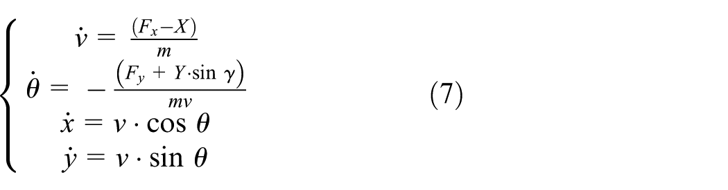
where (x, y) is the position of the UAV, v is the resultant velocity in the 2D horizontal plane, and θ is the heading angle of the UAV. When the heading angle is along with the x, θ = 0, and rotating in counter-clockwise is positive. m is the mass. X and Y are drag and lift forces, respectively. γ is the roll angle. F_x and F_y are the force components in the x and y directions, respectively.

Since the UAVs fly in the horizontal plane, there is no longitudinal maneuver. Then, the lift force has to compensate for the gravity of the aircraft

$$\mathrm{mg}=Y\cos \gamma$$

(8)

If the above expression (8) is introduced into equation (7) and the drag force is ignored, the dynamic model of aircraft can be described as follows

$$\{\begin{array}{c}\stackrel{·}{v}=\frac{\left|F_{\mathrm{total}}\right|·\cos (\phi -\theta )}{m}\hfill \\ \multicolumn{1}{c}{\stackrel{·}{\theta }=-\frac{(\left|F_{\mathrm{total}}\right|·\sin (\phi -\theta )+\mathrm{mg}·\frac{\sin \gamma }{\cos \gamma })}{\mathrm{mv}}}\\ \multicolumn{1}{c}{\stackrel{·}{x}=v·\cos \theta }\\ \multicolumn{1}{c}{\stackrel{·}{y}=v·\sin \theta }\end{array}$$

(9)

Since the UAV is flying in the horizontal plane, at certain position of UAV’s flight path, the radius of turn equals to derivative of path length s to the heading angle θ

$$R_{\mathrm{turn}}=-\frac{\mathrm{ds}}{d\theta }=\frac{v}{d\theta /\mathrm{dt}}$$

(10)

Then, we can obtain

$$R_{\mathrm{turn}}=\frac{m{v}^2}{F_y}$$

(11)

In addition, since the UAV cannot take shape turn, the minimum radius of turn of the UAV, $R_{\mathrm{turn}max}$ , becomes the constraining factor. We assume that the aircraft has sufficient thrust for a sustained turn

$$R_{\mathrm{turn}max}=\frac{m{v}^2}{F_{ymax}}$$

(12)

where $R_{\mathrm{turn}max}$ is a predefined parameter, and it governs the maximum lateral force. Accordingly, constraint of turn radius is mapped into the constraint of maximum lateral force

$$\left|F_{\mathrm{total}}\right|·\sin (\phi -\theta )\le F_{ymax}-\mathrm{mg}·\frac{\sin \gamma }{\cos \gamma }$$

(13)

Thus, we described the derived equations of motion of UAVs in inertial coordinates. These derived equations can make use of Runge–Kutta approach for the orientation model. In our case, we apply four steps Runge–Kutta approach, in that it could get more accurate results than Euler approach, and it is easily programmed for computers. The dynamic model of UAV can be abstracted as follows

$${\stackrel{·}{g}}_i=f(t,g_i),g_i\left(t_0\right)=g_i\left(0\right)$$

(14)

where i = 1, 2, 3, and 4. When i is 1, the above function shows the dynamics of velocity; when i is 2, it shows the motions of the heading angle θ; and when i equals 3 or 4, it shows the changes of positions in x-axis or y-axis. Then, the details of four steps Runge–Kutta method are described as follows

$$\{\begin{array}{c}{g}_{n+1}=g_n+\frac{h}{6}(k_1+2k_2+2k_3+k_4)\hfill \\ \multicolumn{1}{c}{t_{n+1}=t_n+h}\end{array}$$

(15)

For n = 0, 1, 2, 3, …, using

$$\{\begin{array}{c}{k}_1=f(t_n,g_n)\hfill \\ k_2=f(t_n+\frac{h}{2},g_n+\frac{h}{2}{k}_1)\hfill \\ k_3=f(t_n+\frac{h}{2},g_n+\frac{h}{2}{k}_2)\hfill \\ k_4=f(t_n+h,g_n+h{k}_3)\hfill \end{array}$$

(16)

where h is the time step, g_n+1 is the Runge–Kutta approximation of g(t_n+1), and the next value (g_n+1) is determined by the present value g_n plus the weighted average of four increments k₁, k₂, k₃, and k₄.

Alterable potential field method

In this study, we want to utilize potential field method to control the UAVs to execute the path planning in order to achieve the persistent surveillance. Some modifications on the conventional potential field method have to be made. Usually, the primary potential field of driving the UAVs to approach the goal, the attractive potential field, is constant. It is suitable for the one-time mission. In the persistent surveillance task, UAVs require to find another destination when they arrive at the previous predefined goal. In this case, the attractive potential field has to become alterable.

As we defined before, the attractive potential field consists of the magnitude and the orientation. The orientations determine the directions of movement of UAVs, and the magnitudes determine the velocities of UAVs. In this study, we are very interested in whether the UAVs visit each part of the ROI, rather than the time when the UAVs fly over that part. Therefore, we only artificially alter the orientation of attractive potential field, rather than the magnitude.

Tradition to-and-fro scheme

The traditional to-and-fro search pattern for the ROI can also be achieved by designing the alterable potential field rationally. Specifically, the orientation is set toward one side of the ROI. When the UAVs fly in the attractive potential field for a certain interval or arrive at the side, the orientations switch to the opposite side. In this study, we alter the orientation periodically. Although this scheme could extend the straight path and reduce the turning times, it requires the UAV make around 180° turn in each orientation alteration.

Quarter scheme

In order to avoid the 180° turn, we present a quarter scheme: the orientation of attractive potential field is altered 4 times periodically. We use an example to illustrate the quarter scheme. As shown in Figure 2, when the UAV enters the ROI from the side a, the orientation of attractive potential field is heading toward its neighboring side b. When the UAV flies for a predefined interval t₁, the orientation of attractive potential field is altered toward the side c. After an interval t₂, the side d is set as the orientation. When the UAV flies for an interval t₃, the orientation is altered toward the initial side a. After an interval t₄, the UAV flies toward the side b. Therefore, the one complete period consists of four alterations of orientations. The other periods repeat the above process.

Figure 2.

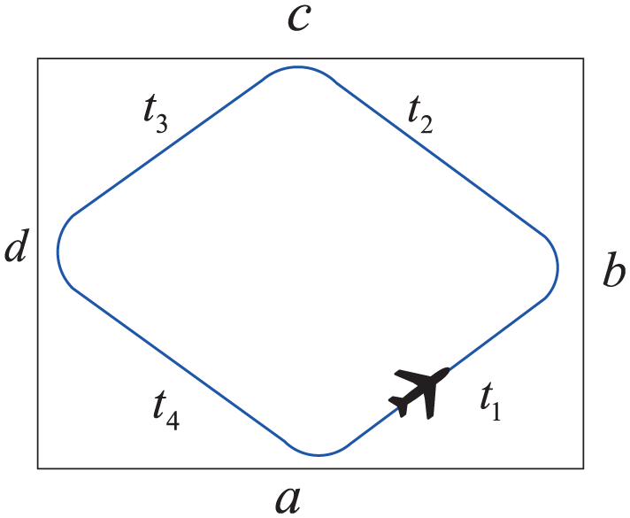
Quarter scheme.

Composite scheme

The two above schemes are well regular essentially. Flexibility and adaptability for environment are absent in these schemes. In this case, we present a composite scheme coupled with the compromise between the turning times and the turning angle. In the first period, the orientation alteration is based on the quarter scheme. The attractive goal is randomly located in any position of the corresponding side. In the second period, the to-and-fro scheme is utilized to alter the orientation. The attractive goal is also randomly scattered in the corresponding side. The rest periods can be set in the same manner.

Where T is the periodicity of orientation alteration, t₁, t₂, t₃, t₄, t₅, and t₆ are the intervals of alteration. Figure 3 shows the changes in orientation of the attractive potential field during the UAVs’ flight.

Figure 3.

Orientation alteration of potential field for UAVs in the composite scheme.

Therefore, we could obtain the overall control flow for path planning of persistent surveillance, as shown in Figure 4. The UAVs are deployed at the beginning. Then, the orientations of the attractive potential are set as one side of the target region which is far away from the initial positions of UAVs. The sensors for sensing obstacles start to work. If any obstacle is sensed, the obstacle-avoidance potential field is generated according to expression (4); otherwise, skip this process. Then, the collision-avoidance and the formation potential are formed for keeping all the UAVs in one group. Till now, all the components of potential field are acquired. They are introduced into the dynamic model of UAVs. Utilizing the Runge–Kutta method, we can estimate the kinematical states of UAVs. Afterward, the process advances a time step. If the current time exceeds the interval, the orientation of attractive potential field is altered according to certain one of the above presented schemes. Then go back to the stage of sensing obstacles.

Figure 4.

Flowchart of path generating by artificial potential field.

Performance evaluations

In order to evaluate the performance of the presented schemes, it is required to make some simulations. All the simulations in this study have been carried out in MATLAB and Visual C++. The specific parameters that are used in the simulation are shown in Table 1. For the reason of reducing the simulation complexity, all the UAVs enter from certain side of the target region. The UAVs tend to survey different regions under the control of the potential field.

Table 1.

Parameters used in the simulation.

Parameter	Value
Area of region	4000 × 4000 m2
Mass of UAV, m	100 kg
FOV of UAV	45°
Velocity, v	10 m/s
Rsensing	100 m
Rsafe	50 m
Rturnmax	20 m
kgoal	0.15
A	2600
B	1200
kformation	15
dformaiton	200 m
Fymax	250 N

UAV: unmanned aerial vehicle; FOV: field of view.

Figure 5 shows the histories of UAVs’ paths based on the three provided schemes. The red polygons represent the obstacles. The paths of UAVs are indicated by different color lines. The solid circles show the original locations of UAVs. In Figure 5(a)–(c), there are three UAVs deploying the region with two obstacles, and in Figure 5(d)–(f), six UAVs are deployed in the region with the same obstacles. It can be observed that the UAVs are able to spread out in the region to cover different areas of the target region time and again by the three schemes. All the UAVs keep the flying path straight as much as possible. When they encounter the obstacles, they make maneuvers to avoid collisions. Therefore, it shows that all the three schemes could achieve the persistent surveillance over ROI with different amounts of UAVs.

Figure 5.

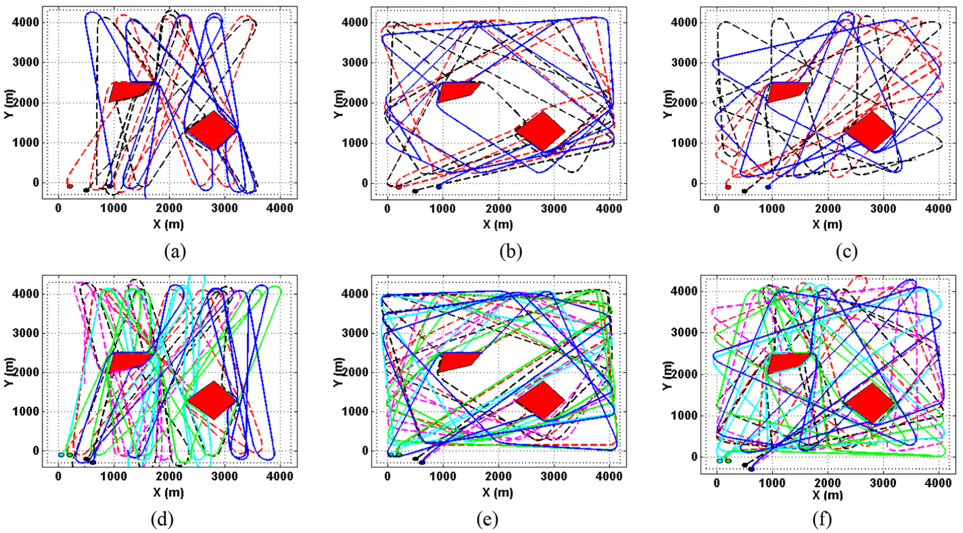
Histories of UAVs’ paths with two obstacles: (a) to-and-fro scheme by three UAVs, (b) quarter scheme by three UAVs, (c) composite scheme by three UAVs, (d) to-and-fro scheme by six UAVs, (e) quarter scheme by six UAVs, and (f) composite scheme by six UAVs.

Figure 6(a)–(c) shows surveillance paths of three UAVs with five different obstacles, and Figure 6(a)–(c) indicates the results of six UAVs with the same five obstacles. The results also demonstrate that all three schemes successfully achieve collision-free flight in the goal of continuous search. Compared with the results in Figure 5, we can obtain that all the three schemes could successfully generate the collision-free paths with different obstacles.

Figure 6.

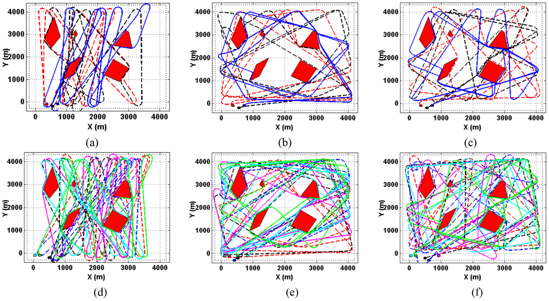
Histories of UAVs’ paths with five obstacles: (a) to-and-fro scheme by three UAVs, (b) quarter scheme by three UAVs, (c) composite scheme by three UAVs, (d) to-and-fro scheme by six UAVs, (e) quarter scheme by six UAVs, and (f) composite scheme by six UAVs.

Moreover, from the results in Figures 5 and 6, we can observe that all UAVs respect the turn radius constraint while changing the directions of flight. In Figure 5, when three UAVs are deployed in the ROI, each UAV takes about eight around 180° turns in the to-and-fro scheme in the simulation time of 4800 s. In the quarter scheme, each UAV takes about 13 around 90° turns. In the composite scheme, each UAV takes about eight 90° turns and four around 180° turns. When six UAVs are deployed in the ROI, each UAV takes about 9 around 180° turns in the to-and-fro scheme, 13 around 90° turns in the quarter scheme, and about 8 90° turns and 4 around 180° turns in the composite scheme. The similar results occur when the UAVs are deployed in the ROI with different obstacles as shown in Figure 6. Therefore, we can obtain that the composite scheme makes successfully trade-off between the turning times and the turning angle.

In fact, we assume that each UAV carries two kinds of sensors: the first kind of sensors, such as cameras which could collect a huge amount of visual data, ³¹ is mounted at the bottom of UAVs, which is responsible for discovering targets in the field of interest (FOI), and the second kind of sensors is mounted in front of UAVs, which is responsible for detecting obstacles in its flight path. We use the disk model to represent the sensing region of the first kind of sensors, and the sector model to represent the sensing region of the second kind of sensor, as shown in Figure 7. R_c is the radius of the sensing circle of the first kind of sensors. R_sensing is the sensing radius of the second kind of sensors. For evaluating the coverage by UAVs, we assume that if the distance between UAV and a point in the target region is smaller than the sensing radius R_c, then this point is absolutely detected by the UAV. In order to evaluate the coverage performance of UAV, we assume that the sensing radius R_c is 70 m. Introducing this sensing model into the trajectory path, we can obtain the coverage of UAVs for the target region.

Figure 7.

Sensing model of UAVs.

The histories of target region coverage by UAVs with two obstacles and five obstacles are shown as the above in Figure 8. The dash lines show the coverage histories when 3 UAVs are deployed, and the solid lines show those when 6 UAVs are deployed. In both cases, it can be observed that the observed area in the target region is getting bigger by all the three schemes with the increase in simulation time, no matter how many obstacles exist in the ROI. As shown in Figure 8, at the initial stage of surveillance, the coverage in the three schemes is almost the same. However, with the time goes on, the coverage in the composite scheme becomes advantageous compared with other two schemes. The coverage of the to-and-fro scheme is worst in the three schemes. Therefore, it could be shown that the composite scheme has better exploit performance for the uncovered area than other schemes. Moreover, from Figure 8, we can also observe that the amount of UAVs influences the performance of persistent surveillance. The large UAVs group obtains the better coverage than the small UAVs group in all the three schemes. We can obtain the similar result when the sensing radius R_c becomes 100 m in the same scenarios, as shown in Figure 9. Besides, we can observe that with the increase in the sensing radius, the coverage percentage of the ROI is getting better. Note that the coverage in the composite scheme with three UAVs displays better performance than that in the to-and-fro scheme with six UAVs.

Figure 8.

History of coverage by UAVs in the scenario with R_c = 70 m: (a) two obstacles in ROI and (b) five obstacles in ROI.

Figure 9.

History of coverage by UAVs in the scenario with R_c = 100 m: (a) two obstacles in ROI and (b) five obstacles in ROI.

Furthermore, we want to acquire not only the covered area in history but also the real-time sensed area. The real-time sensed areas in the to-and-fro, quarter, and composite schemes with two obstacles and five obstacles are shown in Figure 10(a) and (b), respectively. Although at the beginning of simulation, the real-time sensed areas in the three schemes are almost the same, the real-time sensed area in the composite scheme exceeds that in the to-and-fro scheme and quarter schemes in most of the simulation. When six UAVs are deployed in the ROI with two obstacles, shown as the solid lines in Figure 10(a), the average real-time sensed area in the composite scheme is 124,450 m2. In contrast, the to-and-fro scheme has the average real-time sensed area of 112,000 m², and the average real-time sensed area is 119,840 m² in the quarter scheme. The bigger the real-time sensed area, the better we can obtain understanding for the target region. From this perspective, the composite scheme has preferable performance in real-time understanding of the target region. When three UAVs are deployed in the ROI with two obstacles, shown as the dash lines in Figure 10(a), the average real-time sensed areas in the composite scheme, quarter scheme, and to-and-fro scheme are 65,480, 61,120, and 52,460 m², respectively. The big groups of UAVs have larger real-time sensed areas than the small group in all the three schemes. The similar results are obtained when five obstacles are existed in the ROI, as shown in Figure 10(b).

Figure 10.

Real-time sensed area by UAVs: (a) two obstacles in ROI and (b) five obstacles in ROI.

We also change the velocities of UAVs from 5 to 20 m/s in the scenarios with two obstacles and five obstacles. We compare the time when the coverage percentage reaches 90%. The results are shown in Figure 11. Figure 11(a) shows the results when two obstacles exist in the ROI, and Figure 11(b) shows the results when five obstacles exist. It is obviously that the times when the coverage percentage reaches 90% decrease with the increases in velocities in both scenarios. No matter what velocity is and no matter how many obstacles exist, the UAVs could achieve the 90% coverage with the minimum time by the composite scheme. Note that the times when the coverage percentage reaches 90% with the large groups of UAVs are longer than those with the small groups of UAVs.

Figure 11.

Times when the coverage percentage reaches 90% with different velocities: (a) two obstacles in ROI and (b) five obstacles in ROI.

We take the cell-based method ²⁷ as a reference to evaluate the performance of our potential field method. Figure 12 shows the average real-time covered area with different amounts of UAVs using the cell-based method and our potential field method. Figure 12(a) shows the results when two obstacles exist in the ROI, and Figure 12(b) shows the results when five obstacles exist in the ROI. In both scenarios, we can observe that the average real-time covered areas by the cell-based method are the least in the four schemes, no matter how many UAVs are deployed. The underlying reason is that in our method, we design a formation potential field to maintain the distances between UAVs neither too close nor too far. This simulation shows that out proposed method has better performance in real-time coverage compared with the cell-based method.

Figure 12.

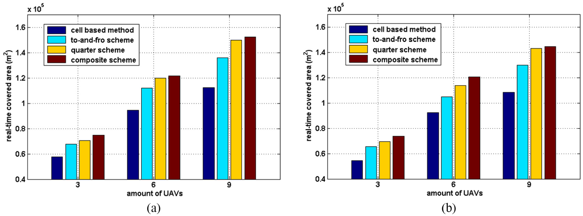
Comparison of real-time covered area by different methods: (a) two obstacles in ROI and (b) five obstacles in ROI.

Conclusion and future work

In this study, we have developed an alterable potential field method for path planning of UAVs in order to realize persistent surveillance. We design three schemes, to-and-fro, quarter, and composite schemes, to artificially alter the directions of potential fields periodically to ensure that UAVs stay over the target region. Under the influence of the potential fields, collision-free paths for executing persistent surveillance are provided, which take the consideration of dynamic constraints of UAVs. The simulation results show that our proposed scheme has preferable performance in exploiting the unobserved area and in real-time understanding of the target region. Future work are oriented to select the optimal amount of UAVs to perform persistent surveillance for a given target region. We also plan to extend our work in the three-dimensional (3D) target space.