Sage Journals: Discover world-class research

Abstract

Aircraft structural damage detection is becoming of increased importance. Technologies such as acousto-ultrasonic have been suggested for this application; however, an optimization strategy for sensor network design is required to ensure a high detection probability while minimizing sensor network mass. A methodology for optimizing acousto-ultrasonic transducer placement for adhesive disbond detection on metallic aerospace structures is presented. Experimental data sets were acquired using three-dimensional scanning laser vibrometry enabling in-plane and out-of-plane Lamb wave components to be considered. This approach employs a novel multi-sensor site strategy which is difficult to achieve with physical transducers. Different excitation frequencies and source–damage–sensor paths were considered. A fitness assessment criterion which compared baseline and damaged data sets using cross-correlation coefficients was developed empirically. Efficient sensor network optimization was achieved using a bespoke genetic algorithm for different network sizes with the effectiveness assessed and discussed. A comparable numerical data set was also produced using the local interaction simulation approach and optimized using the same methodology. Comparable results with those of the experimental data set indicated a good agreement. As such, the numerical approach demonstrates that acousto-ultrasonic sensor networks can be optimized using simulation (with some further refinement) during an aircraft design phase, being a useful tool to sensor network designers.

Keywords

Lamb waves acousto-ultrasonics optimization laser vibrometry local interaction simulation approach structural health monitoring

Introduction

There is increasing pressure on the aviation industry to reduce greenhouse emissions resulting from airline operations. Although the aerospace industry is not currently the greatest contributor,¹ historical trends show that global air travel and hence potential emissions are doubling every 15 years.²

Emissions can be lowered by reducing the mass of the primary structure leading to lower overall fuel burn throughout the aircraft’s operational lifecycle. This can be achieved using adhesive bonding techniques in place of traditional mechanical fastening methods which have increased strength to mass ratios while having improved structural performance and integrity.^3,4 Despite the mass, cost and manufacturing benefits of bonded joints,⁵ there is lack of engineering confidence in their use,⁶ particularly in the hostile environments that the bond will experience (i.e. varying temperatures, water ingress and high levels of humidity).^7–9 This has led to over engineered, heavy design solutions¹⁰ typically using adhesives combined with arrestment fasteners.¹¹

Past failures of in-service adhesively bonded joints^12,13 have demonstrated that regular monitoring of the bonded joints is required to ensure structural integrity. It is proposed that an ‘as required’ inspection program could be employed through the installation of a structural health monitoring (SHM) sensor network which has many advantages over traditional non-destructive testing (NDT) techniques¹⁴ as well as delivering mass savings if designed concurrently with the aerostructure.¹⁵

Acousto-ultrasonic (AU) induced Lamb waves are a long-established technique for detecting damage in structures.^16,17 The technique involves exciting a transducer mounted to the structure, inducing a Lamb wave which is sensed by another transducer mounted elsewhere on the structure. If damage occurs at any point in the source-sensor path, the wave propagation is altered resulting in a quantifiable difference in the signal received.

Sensor network design is an important consideration for ensuring a high probability of damage detection and structural integrity while ensuring additional weight penalties (from redundant sensors), power demands and computational requirements are minimized.

Many studies to optimize SHM sensor networks have been conducted but few use an empirical approach, particularly for the optimization of AU sensor networks. Genetic algorithms (GAs) have been widely used for optimizing the placement of sensors because of their ability to converge on the global optima.^18–20 Guo et al.²¹ used an improved GA to assess the fitness derived from a Fisher information matrix for placing strain gauges on truss structures to identify changes in stiffness caused by damage in a finite element model. Worden and Burrows¹⁹ applied a neural network technique to classify damage and optimize sensor locations from a finite candidate set on a cantilever plate. Optimization was achieved using curvature algorithms, simulated annealing and GAs which showed consistent agreement, although it was stated that the GA showed greatest potential. A Bayesian approach to minimize type I or type II (false positive or false negative) errors was applied to optimal sensor placement of an active SHM system by Flynn and Todd²² for simplistic structures. A GA was used to search the global optimality criterion achieving sensor networks which maximized the probability of detection and reduced the probability of a false alarm. Gao and Rose²³ used a covariance matrix adaptation evolutionary strategy to optimize sensor locations for ultrasonic guided wave networks on realistic aircraft structures. This novel technique showed performance gains over random networks, identifying areas of high probability of damage producing a sensor network that provided a suitable trade-off between miss-detection probability, number of sensors and performance.

Downey et al.²⁴ developed an optimal placement strategy for the placement of strain gauges within a hybrid dense sensor network to monitor local changes of in-plane strain over a global area. A multi-objective approach was taken to reduce the occurrence of type I and type II error which was formulated as a single objective problem by linear scalarization. This was interrogated by a learning gene pool GA and the optimal placement of the sensors was verified experimentally for known load cases.

Fang et al.²⁵ tackled the problem of optimal modal sensor placement for wireless sensors using a cluster-based approach with the objective of reducing power used by the network for monitoring truss structures. Studies were conducted both experimentally and numerically with the network optimized by a GA. Using this approach, the power demands of the system were able to be reduced when compared to previous approaches.

Huang et al.²⁶ applied GAs to find the optimal number of temperature and strain sensors for monitoring structures in harsh environments. The network was optimized for numerical and experimental scenarios with considerations for a trade-off between cost and measurement accuracy. A good agreement was found between the numerical and experimental studies.

This article begins by presenting a description of an experimental investigation into AU sensor location for the monitoring of an adhesively bonded stiffener with and without a disbond. The results of an optimization study based on the use of a GA are then presented with consideration of both the out-of-plane and in-plane components of the Lamb waves. With a view to developing a network design technique to be used as part of the component design process, a computational model of the same adhesively bonded component is conducted using a local interaction simulation approach (LISA). The results from optimization using the modelled data are then presented and explored, drawing comparisons between the experimental and computational investigations. A series of recommendations are then made on how the methodology presented could be used for the concurrent design of a structure and sensor network.

Experimental setup

3D scanning laser vibrometry was used to obtain the experimental data set to optimize AU sensor locations on a stiffened aluminum panel.

Panel manufacture and geometry

A 3 mm 6082-T6 aluminum alloy plate was bonded using commercially available Araldite^® 420 adhesive to a 6082-T6 aluminum alloy unequal angle stiffener to construct the stiffened panel, as shown in Figure 1.

Figure 1.

Dimensions of the stiffened panel, excitations sites and scan area (all dimensions in millimeter).

The dimensions of the panel were chosen to reduce the effects of edge reflections. The film thickness of the adhesive was regulated using 0.1 mm copper wire gauges, achieving optimal shear strength following manufacturer’s recommendations.²⁷

A geometrically similar second panel with an induced disbonded region of 25.4 mm in length at the centre of the stiffener, across its width, was also manufactured. PTFE tape was installed to induce the disbonded region prior to applying the adhesive. The tape was removed once the adhesive had cured. A square region of 625 mm × 625 mm in the centre of each panel on the face with the stiffener was designated the investigation region, as shown in Figure 2.

Figure 2.

Layout of the area of investigation.

A commercially available PANCOM Pico-Z (resonant band 200–500 kHz) transducer was acoustically coupled to the panel using Loctite^® Ethyl-2-Cyanoacrylate adhesive at the five excitation sites on the left-hand boundary of the investigation region shown in Figure 1. Multiple excitation sites enabled the effectiveness of the transducer-disbond path to be investigated, in effect simulating different disbond positions relative to a single transducer site. The distance of the left-hand boundary to the stiffener was selected to reduce the effects of edge reflections on the transmitted wave while also allowing sufficient distance from the measurement, ensuring Lamb waves had fully formed.²⁸ The transducer used was selected because of its flat, broadband response in the frequency range under investigation (200–500 kHz) and its relatively small face, making it more representative of a point source. A photograph of the experimental setup is presented in Figure 3.

Figure 3.

Experimental setup.

Experimental parameters

A 10-cycle sine burst was generated by Mistras Group Limited (MGL) WaveGen function generator software connected to MGL μdisp/NB-8 hardware. A 160 V peak-to-peak excitation amplitude was used to create high velocity Lamb wave oscillations. Three excitation frequencies were selected for this experiment: 100, 250 and 300 kHz, to investigate the interaction of a range of wavelengths (presented in Table 1) with the defect.

Table 1.

The calculated wavelengths for each excitation frequency.

Frequency (kHz)	A₀ wavelength (mm)	S₀ wavelength (mm)
100	15	55
250	9	22
300	8	18

Although the 100 kHz excitation fell outside of the resonance range of the sensor, it had previously demonstrated useable results.²⁹ A 10 V peak-to-peak signal was also generated and used as a reference for triggering the acquisition of the vibrometer. A repetition rate of 20 Hz was used, giving sufficient time for the induced wave energy and reflections to fully dissipate before taking the next measurement.

A Polytec PSV-500-3D-M vibrometer with three laser heads was used to measure the in-plane and out-of-plane vibration components at each scan point. As measurements are taken by three heads, it is less important for the laser heads to be perpendicular to the structure under test than with a 1D system. A sampling frequency of 2.56 MHz per channel was used which gives sufficient resolution for reconstructing the wave with a high level of fidelity (hence excitation frequencies above 300 kHz were not considered due to the constraint of the maximum sampling frequency of the vibrometer). To increase the signal-to-noise ratio, 200 measurements at each point were taken and the signals were averaged.

825 vibrometer measurement points were set up within the investigation region (as shown in Figure 2) which was coated with retro-reflective glass beads to improve the back-scatter of the laser light and hence the quality of the signal. No measurement points were positioned within a 25 mm wide region on either side of the stiffener due to the positioning of the laser heads which resulted in the stiffener casting a shadow where it was impossible for all three lasers to align. There were also no measurement points positioned in a 78 mm wide region to the right of the excitation sites as shown in Figure 1 to save acquisition time as preliminary tests had demonstrated insignificant findings in this region.

During testing, each panel was laid on ‘bubble wrap’ to acoustically uncouple it from the floor. Measurements were taken on each panel using the laser vibrometer to produce two data sets, with and without the induced disbonded region. Positioning relative to laser head was ensured by a series of markers laid within the laboratory and on the panels. A low-pass front end filter was set at 20 kHz above the excitation frequency to filter out high-frequency noise.

Signal processing

In order to determine the presence of damage, and hence develop a metric to establish the optimal sensor positions, the signals measured by the vibrometer were post-processed using a comparative technique.

Integration

The laser vibrometer measures the velocity of the wave whereas sensors bonded to the structure typically measure the displacement. In order to make this optimization study more representative of the input received by sensors bonded to the structure, all velocity signals were integrated to obtain the displacement signals.

Cross-correlation

The cross-correlation technique has been proven to be a successful statistical method for quantifying differences between two waveforms and is therefore well suited to identifying the presence of damage in an AU system.³⁰ Typically, a value of unity for the cross-correlation coefficient indicates that the received waves are identical, and hence, there is no damage present. A value less than unity identifies differences in the waveforms and thus the likely presence of damage.

By calculating the cross-correlation coefficient for the out-of-plane component of the Lamb wave for each measurement point (with and without the induced disbonded region – example waveforms presented in Figure 4), it was possible to produce five data sets (one for each excitation site). It is evident from visual inspection of the waveforms in Figure 4 that they are different; thus, a cross-correlation coefficient of 0.7445 was calculated due to the presence of the disbonded region. For further comparison of the waveforms and the influence of the stiffener, the reader is referred to the authors’ previous work.²⁹

Figure 4.

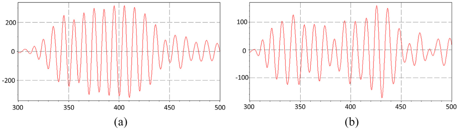
Comparison of out-of-plane waveforms from a measurement point to the right of the stiffener, in-line with excitation site 3: (a) healthy panel and (b) panel with the disbonded region.

Figure 5 shows the cross-correlation coefficients at each measurement point for the 100 kHz excitation at excitation site 3, demonstrating areas of low cross-correlation coefficient resulting from the presence of the disbond. The out-of-plane component of the Lamb wave was primarily considered as it is the principle component being excited and sensed by bonded transducers.

Figure 5.

Cross-correlation plot for excitation site three (100 kHz excitation). The location of the excitation is denoted by the blue circle.

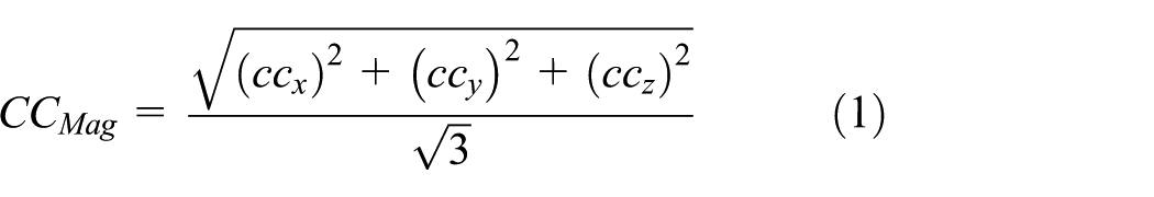
Three-component cross-correlation

The x, y and z components of the wave at each measurement point were acquired. In order to enable the optimization algorithms to consider all three components, the vector sum of the cross-correlation coefficients was calculated and divided by √3, as shown in equation (1), making the results comparable with the out-of-plane results

C C_{Mag} = \frac{\sqrt{{(c c_{x})}^{2} + {(c c_{y})}^{2} + {(c c_{z})}^{2}}}{\sqrt{3}}

(1)

Time window

The data sets (with and without the induced disbonded region) were originally correlated for the entire sample length of the measurements (1.6 ms). This however produced low cross-correlation coefficient values at all measurement points due to the reflections and refraction patterns caused by the disbond. To improve the correlation, a 200 μs time window was used, capturing mainly the transmitted wave, reducing effects of reflection. The start of the time window was determined by an amplitude threshold value of 40% of the maximum amplitude value in the first 700 μs of the entire sample length for each respective measurement point of the data set without the disbonded region. The 40% threshold level was determined by assessing the peak of the first wave received (the first wave received was lower than the peak due to transducer inertia) while ensuring that it was not triggered by any background noise which was found to work well. A 14% pre-trigger was applied at the point which the wave amplitude crossed the threshold, ensuring that the start of the transmitted wave was captured, to determine the start of the window as demonstrated in Figure 6.

Figure 6.

Example out-of-plane waveform to demonstrate how the time window was determined.

Optimization

Using each cross-correlation data set for each excitation site, it was now possible to form a methodology for the optimization of the sensor locations. On reviewing the literature, the authors are not aware of any studies that adopt an optimization strategy using waveforms from healthy and damaged structures based on empirical AU data, as presented.

One fundamental issue with any optimization problem is the design of the fitness function (also known as a cost function, or objective function) to interrogate when seeking optimal solutions. In this case, the fitness function needed to assess the performance of a sensor placed at a discrete location to detect damage from any excitation site.

Fitness function

Each sensing location had five cross-correlation coefficient values (one for each excitation site). In the case of a one-sensor network, it was possible to calculate the fitness of a sensor location using the fitness function shown in equation (2)

Fitness = 1 - (σ + \sqrt{\frac{1}{5} \sum_{i = 1}^{5} x_{i}^{2}})

(2)

where σ is the standard deviation and x is the cross-correlation coefficient.

The aim of the fitness function was to find a sensing location that had low and consistent cross-correlation coefficients regardless of excitation site and hence the greatest sensitivity to damage regardless of source–damage–sensor wave path, representing damage being at different locations on the stiffener relative to the source and the sensor.

To consider multi-sensor networks, a ‘pseudo-sensor’ was created by selecting the lowest cross-correlation coefficients from the sensors in a proposed network for each excitation site and then combining them. This ‘pseudo-sensor’ was then used to calculate the fitness for that particular sensor network as demonstrated in the case of a two-sensor network in Table 2.

Table 2.

Cross-correlation coefficient for a two-sensor network.

	Excitation sites
	1	2	3	4	5
Sensor A	0.8087	0.6007	0.7355	0.6502	0.8791
Sensor B	0.6412	0.9576	0.6435	0.8222	0.5681
Pseudo sensor	0.6412	0.6007	0.6435	0.6502	0.5681

The numbers in bold are used to create the pseudo sensor.

To avoid redundant sensors (i.e. sensors that do not contribute any cross-correlation coefficients to the ‘pseudo-sensor’), each network was checked to ensure all sensors in the network were used. If redundant sensors were found, an artificially low fitness was assigned to that sensor network which ensured it would not be identified by the optimization algorithm.

Optimization problem

The number of possible sensor network combinations increases with the network size by a multiple of the respective binomial coefficient. In this study, the number of candidate sensor locations was 825, arranged in a regular square grid within the investigation region shown in Figure 2. The number of possible sensor combinations is shown in Table 3 for networks of up to five sensors. Evaluating the effectiveness of every possible solution would have been computationally expensive, ruling out simplistic techniques such as an exhaustive search.

Table 3.

The number of sensor network combinations for a given number of sensors in the network.

Number of sensors in network, N_s	Number of possible sensor network combinations
1	825
2	339,900
3	93,245,900
4	1.92 × 10¹⁰
5	3.15 × 10¹²

GAs

GAs are an optimization technique developed by Holland³¹ based on the theory of evolution. Each ‘generation’ of solutions includes more suitable and less suitable solutions. The less suitable are discarded in a manner analogous to Darwinian evolution.

GAs have advantages over other optimization techniques as they have the ability to interrogate the whole search space to find the global minimum or maximum rather than converging on local minima or maxima. The algorithm, which is outlined in Figure 7,²⁹ interrogates a relatively low proportion of the total search space and therefore is not as computationally expensive as other techniques.³³ A brief overview of a GA is presented here. For further explanation, the reader is referred to Haupt and Haupt.³³

Figure 7.

Schematic representation of a GA (recreated from Clarke and Miles³²).

GA configuration

For this study, binary encoding was used. Each candidate sensor location was assigned a numerical value (i.e. locations 1-825) which was encoded into a binary string (known as a ‘gene’). Each sensor in the network contributed to the full binary string (known as a ‘chromosome’) which described one candidate sensor network within the population of solutions as shown in Figure 8. The chromosomes were used by the algorithm for mating and mutation when producing the next generation of solutions.

Figure 8.

Definition of the terms used in binary encoded genetic algorithms.

A 10-digit binary string was required in order to assign each candidate location. As 825 is not the maximum 10-digit binary number, it was possible for the GA to create a solution outside of the range of physical locations. To resolve this, penalty values were assigned to binary values representing locations greater than 825 hence assigning poor fitness to solutions containing these genes, leading to them being discarded by the GA. The initial population used was 40 times the number of sensors in the network ensuring a suitable subset of the population was considered without having a detrimental effect on the optimization algorithm’s performance, based on prior experience. The initial population size was increased as the size of the search space increased in order to ensure sufficient sampling.

A simple pairing technique where the two best solutions in the population were selected for mating, followed by the next best two until the whole mating pool had been paired up was used. A randomly assigned cross-over point was used for each mating pair giving a good ability to carry forward the best attributes of the solution without continuously producing poor solutions which can be a drawback of fixed point cross-over schemes.³³

An allele mutation was adopted for this GA to explore the search space and prevent convergence on a local maxima. A uniform probability of mutation of 0.1 was used for this problem as good results in a previous, preliminary study demonstrated search space exploration with convergence on the global maxima.³⁴ The fittest 10% of solutions were made immune from allele mutation which prevented good solutions being mutated into poorer solutions, and hence being discarded.

As with all GAs, confirmation of convergence can prove difficult as there is no indication that the optimal solution has been reached; a drawback of a GA as every solution is not exhaustively considered. In this study, a solution was deemed to be optimal when the fittest solution had not been improved upon for 2000 generations, an approach previously found successful.²⁹

Optimization results from experimental data

Out-of-plane Lamb wave component

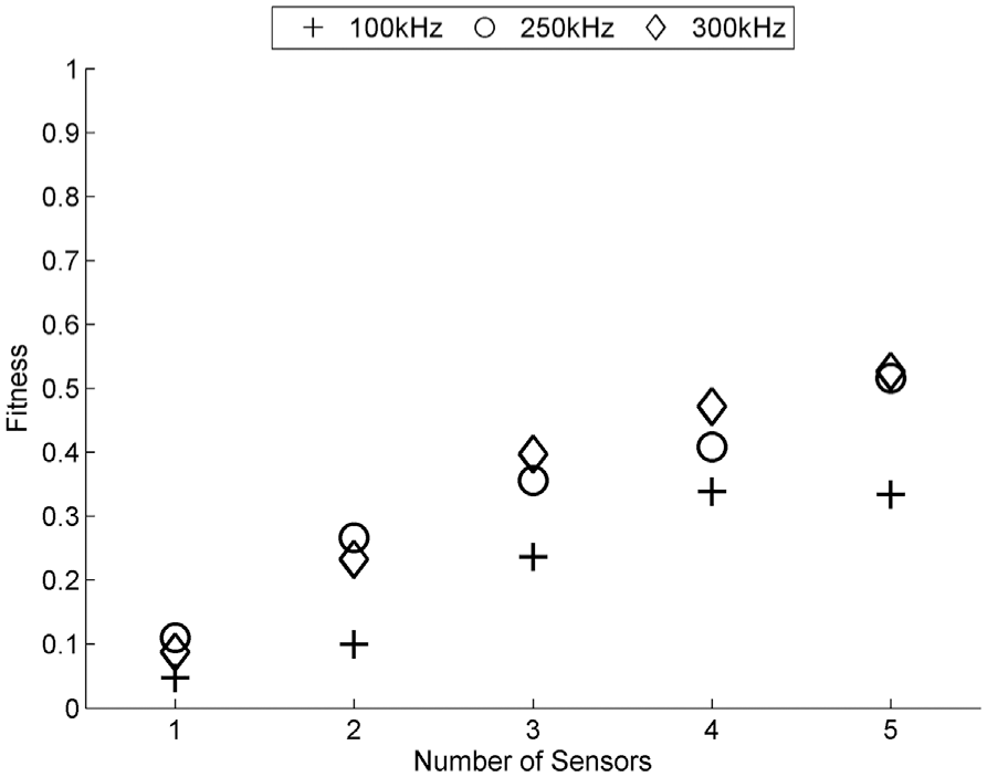
The optimal fitness against sensor network size for the out-of-plane component at each excitation frequency is presented in Figure 9.

Figure 9.

Calculated fitness for each number of sensors in a sensor network at the three excitation frequencies for the out-of-plane component of the Lamb wave.

It is apparent that as the excitation frequency increases, there is a significant increase in fitness demonstrating greater damage sensitivity of higher frequency waves due to the shorter wavelengths (the wavelengths of both modes reduce as the frequency increases as shown in Table 1). At 300 kHz, the wavelength of the S₀ mode is comparable to that of the A₀ mode of the 100 kHz excitation, meaning both modes are more sensitive to the damage.³² This is supported by the visual representations in the authors’ earlier work²⁹ However, as the excitation frequency increases, the received signal is more susceptible to noise due to the material’s microstructure scattering the wave.³⁵ Random noise would reduce the cross-correlation coefficient though not to the extent presented here – hence damage has been detected. Attenuation of the wave increases with excitation frequency resulting in a greater reduction of amplitude as the wave propagates which is an important consideration for sensor network design and selecting appropriate excitation frequencies.

These results also show that fitness increases as the number of sensors in the sensor network increases demonstrating that more sensors in the network improve damage sensitivity. With the 100 kHz excitation, the fitness more than doubles as the network size increases from one to two. Fitness increases at a constant rate as the network size increases from two to four where maximum fitness is achieved. A small reduction in fitness is observed with the addition of a fifth sensor due to the optimization algorithm being forced to use five independent sensors.

A large increase in fitness is achieved with the 250 kHz excitation over the 100 kHz excitation. Comparing the respective one-sensor networks, a fitness over three times greater is achieved. Improvements in fitness are observed as the network size increases to two and again to three. However, minimal increases in fitness are observed in larger sensor networks indicating a three-sensor network to be sufficient for this particular application.

The best fitness was achieved with the 300 kHz excitation. Small improvements in fitness were achieved by increasing the network size from one to two. However, marginal gains were achieved with larger network sizes indicating that a two-sensor network was sufficient when using a 300 kHz excitation frequency.

Sensor location results

The locations for each optimal sensor network are presented in Figure 10. The excitation locations (denoted by the black dots on the left-hand side), the stiffener (denoted by the dashed line) and disbonded region (denoted by the thick black square) are included for completeness.

Figure 10.

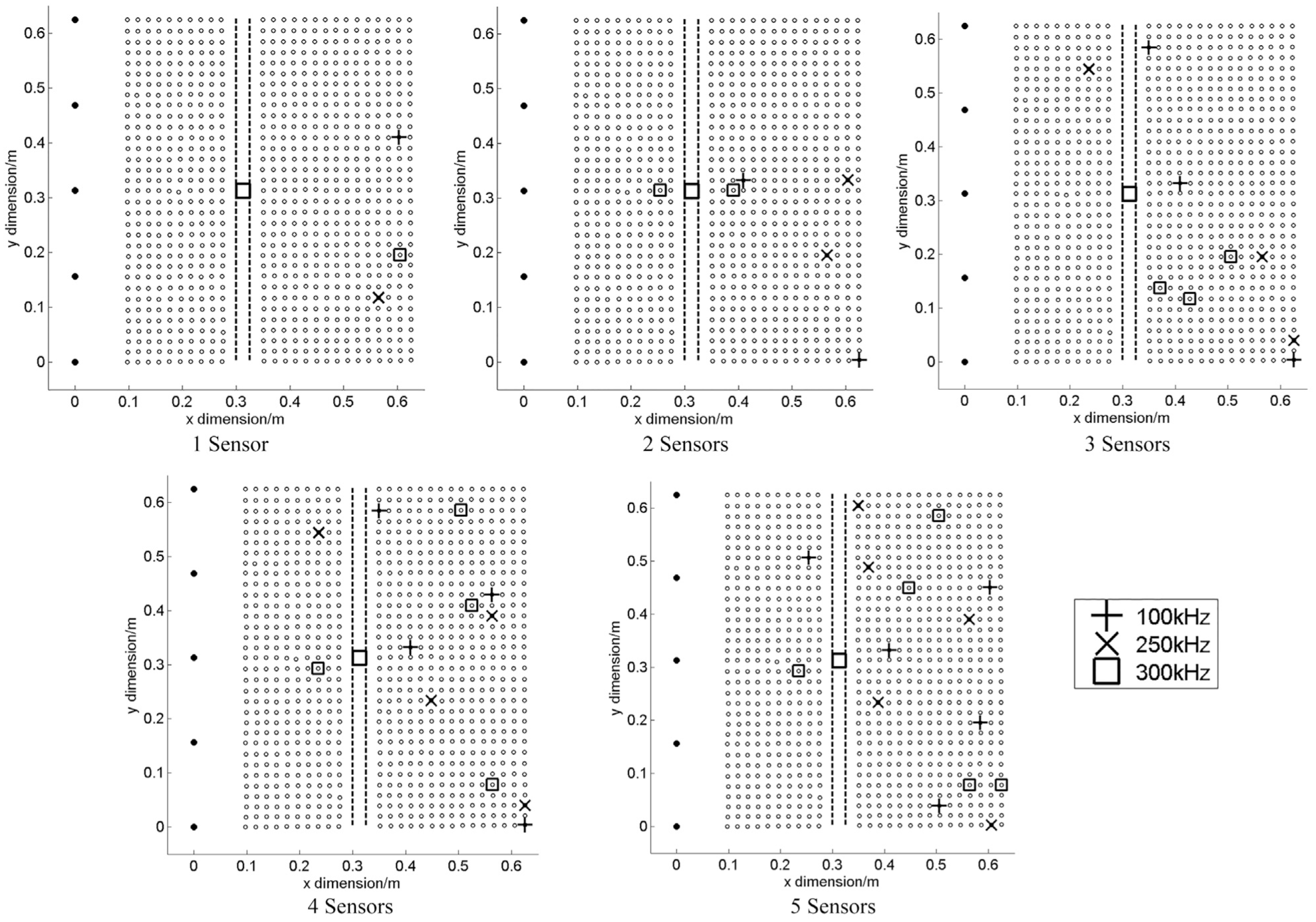
Optimized sensor locations based on the out-of-plane component for all three excitation frequencies.

Sensors were positioned by the optimizer to the right of the stiffener either above or below the disbond for each excitation frequency for a one-sensor network. Previously published results³³ indicate that Lamb wave interaction with the disbonded region produces a diffraction pattern and as such would result in low cross-correlation coefficients in the regions where these sensors have been placed.³⁴

The placement of the two-sensor network places the majority of the sensors in-line with the disbonded region. One sensor for the 100 kHz excitation was placed in the lower right-hand corner which is likely to be due to the diffraction pattern. A similar case is observed with the 250 kHz excitation. Considering the 300 kHz excitation, a sensor was placed in-line with the disbonded region either side of the stiffener which was likely to be caused by reflections from the disbonded region causing differences in waveforms.

The three-sensor networks produced a much wider spread of sensor placement. The 100 kHz excitation results saw a spread of sensors along the length of the stiffener which is likely to be due to differing diffraction patterns from the different excitation sites. A similar distribution of sensors was also placed for the 250 kHz excitation, although one sensor was placed on the left of the stiffener, most likely resulting from reflection fringes. The placement of the sensors for the 300 kHz excitation positioned all three sensors in the lower right quadrant which is unconventional but thought to be the result of complex interaction fringes.

As the network size increases to four, the sensors tend to be distributed along the length of the stiffener. The 100 kHz excitation reuses all sensors from the three-sensor network, demonstrating the strength of these sensing locations. The addition of the fourth sensor however significantly improves the fitness as shown in Figure 9. A similar distribution of sensors was also achieved with the 250 kHz results with sensors widely spread and two sensors carried over from the three-sensor network. The 300 kHz excitation gave near uniform distribution along the length of the stiffener with all but one sensor placed on the right of the stiffener.

Expanding the network to five sensors draws some similarities between the excitation frequencies. The 100 kHz excitation places three sensors in a triangular array mimicking a diffraction fringe similar to that seen in Figure 5 with additional sensors placed above and below these sensors, albeit one on the left of the stiffener. A contrasting triangular placement array was produced with the 250 kHz excitation, although a good distribution of sensors was placed along the length of the stiffener. Increasing excitation frequency to 300 kHz produced three groups of sensors: two above, two below and one in-line with the disbonded region. The sensor placed in-line was placed on the left of the stiffener further demonstrating good sensitivity to the damage in this region.

Three-component magnitude of the Lamb wave

The fitness against sensor network size for the three-component magnitude is presented in Figure 11 for each excitation frequency. As with the out-of-plane results, increasing the excitation frequency improved the fitness. As previously stated, this is likely due to the smaller wavelengths being more sensitive to the damage.

Figure 11.

Calculated fitness for each number of sensors in a sensor network at the three excitation frequencies for the three-component magnitudes of the Lamb waves.

For all excitation frequencies, there is a trend that as more sensors are added to the network, the fitness improves. For the 100 kHz excitation, a 64% improvement in fitness can be achieved as the network size is increased from one to two. A more linear trend is observed as the network size is increased from two to five, although the improvement in fitness is not as significant as the improvement from one sensor to two. It is likely that further increasing the network size would deliver ever diminishing improvements in performance.

As the network size is increased from one to two for the 250 kHz excitation, there is a 9% increase in fitness. The single-sensor solution fitness is further improved by 16% as the network size increases to three sensors. As the network size is further increased, the improvement in fitness reduces somewhat, with a minimal fitness improvement achieved with a five-sensor network over a three-sensor network.

A similar trend was observed with the 300 kHz excitation as the 250 kHz excitation. A fitness improvement of 15% was achieved by increasing the network size from one to two. This was further improved by the three-sensor network which achieved an increase of 21% over the one-sensor network. Although the best fitness was achieved with the five-sensor network, minimal improvement was achieved over a three-sensor network indicating that this as a sufficient network size in this case.

Discussion

It is evident that increasing the excitation frequency improves the fitness of the sensor networks for both the out-of-plane and three-component magnitude cases. 300 kHz delivered the fittest solutions although, due to experimental constraints, excitation frequencies greater than this were not considered so therefore it is not possible to determine whether higher excitation frequencies would yield further improvements in fitness. It could be inferred however that diminishing fitness improvements may be achieved as a large improvement was observed between the 100 and 250 kHz excitations but not so large an improvement was seen between 250 and 300 kHz excitations. This may be representative of the increments between the excitation frequencies being different.

Although higher excitation frequencies have been shown to perform better, attenuation should also be considered as part of the sensor network design as higher frequency Lamb waves exhibit higher attenuation. This will require a higher density of sensors in order to cover a large structure. This creates a problem of determining the optimal excitation frequency versus the minimum defect size detectable. This promotes the requirement for concurrent design of the structure and sensor network as it may be viable to make the structure damage tolerant in more critical areas while focusing monitoring to areas where there is a high probability of damage.

Computational and power overheads also need to be considered for an installed sensor network when selecting the excitation frequency as a higher sampling rate will be required to reconstruct the wave. This consideration falls outside the scope of this study but is nevertheless important for sensor network design, particularly for a self-powered system.

Considering all three components of the wave improved the sensor network performance with a 72% improvement in fitness of the 100 kHz single-sensor network when compared with the corresponding out-of-plane results. Less significant improvements were observed when using the higher excitation frequencies with fitness improvements of 8% and 11% for the 250 and 300 kHz excitations, respectively, over those of the corresponding out-of-plane five-sensor networks.

Performance has been shown to improve when considering in-plane components; however, sensors tend not to sense solely either in- or out-of-plane due to Poisson’s ratio but do tend to be biased. To improve the methodology presented, it would be useful to model a sensor with known characteristics. It may be advantageous in some scenarios for instance to sense primarily in-plane to reduce the number of sensors while still enabling the same sensitivity to damage.

Disbond damage has only been considered in this study, whereas in-service structures are subjected to many damage events such as fatigue, impacts and corrosion. It would be beneficial for any optimization algorithm to take into account within its fitness function the likelihood of such an event occurring within different regions of the structure enabling a much more robust sensor network to be created.

With both result sets, diminishing returns are achieved as the sensor network increases to a point where there are insignificant gains in fitness. The out-of-plane results suggest that insignificant gains are made by increasing the sensor network sizes beyond four, three and two sensors for 100, 250 and 300 kHz excitations, respectively. Although one-sensor networks in each case detected the presence of damage, improved sensitivity was achieved with additional sensors as well as establishing some redundancy in the system. Therefore, a three-sensor network would provide a suitable level of coverage regardless of excitation frequency for this scenario. However, more sensors may need to be added for a more geometrically complex structure as features on the structures may attenuate the waves, reducing the effective area that can be monitored, hence demonstrating the usefulness of a numerical tool.

Considering the in-plane components, a continual improvement was observed with the 100 kHz excitation, although the biggest improvement was observed between one- and two-sensor networks. The same was observed with the 250 and 300 kHz excitations but with minimal improvements achieved with networks larger than three.

A constant time-window size was used for the cross-correlation analysis for consistency. However, it would be beneficial to tailor this for the shorter duration of the higher excitation frequencies which would reduce effects from edge reflections. A simple thresholding technique was used to determine the start of the time window; however, techniques such as the Akaike information criterion (AIC) have been shown to exhibit good performance in determining the arrival of a wave.³⁶ Adopting this technique would establish a more refined window and reduce misplacement of a sensor.

LISA

The experimental study has only considered one disbond scenario (although different excitation site-disbond paths and angles were considered by having multiple excitation sites). On real aircraft structures however disbonded regions vary in both shape and size which will influence Lamb wave interaction and therefore sensor placement. An extensive experimental program for each scenario would be prohibitively time-consuming and costly; therefore, a simulation tool would be advantageous from a design perspective by enabling sensor network designers to model different damage scenarios in order to determine optimal sensor placements on the structure.

The LISA is a finite difference method which uses sharp interface modelling to solve issues regarding boundaries and discontinuities,³⁷ developed in the early nineties^38–40 for the bespoke purpose of simulating Lamb wave interaction. Since its introduction, there has been much research assessing the accuracy and reliability of models^41–48 which have been validated in experimental studies using laser vibrometry, particularly at boundaries, structural features and defects. LISA has been shown to be well suited to, and is now an established method for, modelling Lamb wave interaction.^38,49–53 For further detail regarding LISA, the reader is referred to Lee and Staszewski.⁵²

In recent years, with the widespread development and use of NVIDA^® CUDA parallel computing architecture, LISA has proven to be an effective way of modelling Lamb wave interaction due to its ability to process large simulations in minutes,⁵⁴ making LISA well suited to modelling different damage scenarios in a short period of time.

Global mesh size

Commercially available MONIT SHM cuLISA3D v0.8.4 was used for this study which has many advantages including a user-friendly interface with MATLAB. One drawback of this version is its adoption of a global mesh size for the entire 3D finite difference model meaning that the model is defined by its smallest dimension (as opposed to other numerical techniques where the mesh can be refined in regions of interest while adopting a coarser mesh elsewhere for computational efficiency). To accurately model the experimental study, the smallest dimension is the adhesive film thickness (0.1 mm). However, using a 0.1 mm global mesh size generated a very large set of cube geometry data (∼20 GB) which was not possible to process on the CUDA graphics card used because of insufficient memory (2 GB). Therefore, the model was simplified to reduce the memory required using a global mesh size of 0.5 mm with dimensions being rounded to the nearest 0.5 mm.

Model setup

To reduce computational overheads, only the area of investigation (outlined in Figure 1) was modelled with the excitation sites modelled on the left-hand boundary to reduce edge reflections, taking the same approach used by Lee and Staszewski.⁵¹ The same excitation frequencies were used for the model as for the experimental study.

The co-ordinates of the sensing locations were exported from the vibrometry software to ensure consistency and rounded to the nearest 0.5 mm for assignment to the corresponding location on the model. The sensing locations were modelled as points representing the point measurements of the laser vibrometer study. An installed sensor would have a face which covers an area; however, this varies for different sensors and falls outside the scope of this study.

A sampling frequency of 20 MHz was used for the model as this had been shown to produce representative results in a previous study⁵⁵ while also ensuring that Courant stability criterion was satisfied.⁴⁵ For consistency, x, y, and z components for a 1.6 ms sample length were recorded at each sensor location.

The plate and the stiffener were given the properties of 6062-T6 aluminum alloy. Due to the global cube edge length constraint, the adhesive layer was not modelled. Instead, the plate–stiffener interface was modelled as a continuous structure which had delivered promising results in a previous study.⁵⁵

Modelling the disbonded region

Given that it was not possible to model the adhesive layer, an alternative solution was adopted to model the disbond. A localized area (25.5 mm × 25.5 mm – rounded to the nearest 0.5 mm due to the global cube edge length constraint) of reduced stiffness in the structure at the location of the disbonded region was created by removing the cubes at the plate–stiffener interface. This technique produced representative results which were presented in Marks et al.⁵⁵

Optimization results from modelled data

The LISA model was used to generate data representative of the experimental study. This was then optimized using the same strategy used in the previous section.

Out-of-plane component of the Lamb wave

The optimal fitness against sensor network size for the out-of-plane component at each excitation frequency is shown in Figure 12.

Figure 12.

Fitness against the optimal network configurations for a given number of sensors using the out-of-plane data from the LISA model.

As with the experimental results, the excitation frequency had a significant influence on fitness, although the best fitness for the one- and two-sensor networks was found with the 250 kHz excitation and not 300 kHz excitation. There was also not as significant a fitness increase between the 100 kHz excitation and the higher frequency excitations when compared to the experimental results.

The poorest fitness was achieved with the 100 kHz excitation using a single-sensor network while the best performance was achieved with a four-sensor network. A small reduction in fitness occurred as the network grew to five sensors as observed in the experimental study. A similar trend in fitness increase was also observed between the two- and four-sensor networks to that seen in the experimental study albeit at a lower overall fitness.

The fittest solutions for the 250 and 300 kHz excitations were achieved with a five-sensor network. A significant increase in fitness was achieved with the 250 kHz excitation as the network grew from one to two sensors. The rate of fitness improvement diminished as the network size continued to grow, although a leap in fitness was observed between four and five sensors.

The 300 kHz excitation showed an almost linear fitness increase as the network size grew from one to three sensors when the 300 kHz excitation out-performed the 250 kHz excitation. Increasing the network size further saw fitness improvements of diminishing returns.

Three-component magnitude of the Lamb wave

The optimal fitness against sensor network size for the three-component magnitude at each excitation frequency is presented in Figure 13.

Figure 13.

Fitness against the optimal network configurations for a given number of sensors using the three-component magnitude data from the LISA models.

As with the out-of-plane results, the higher frequency excitations out-performed the 100 kHz excitation. As the network size increased, a near linear, gradual increase in fitness was achieved using a 100 kHz excitation with an improvement of 150% achieved by a four-sensor network over a one-sensor network. Increasing the network size to five sensors saw a further increase in fitness of 29% over the four-sensor network. The near linearity of these results does not aid in suggesting an optimal sensor network size.

Similar fitness increment trends were observed by both the 250 and 300 kHz excitations as the network size grew. Progressive fitness increases were observed for both excitations between networks of one and three sensors; however, larger networks yielded minimal (if any) increases in fitness demonstrating little performance to be gained; thus, suggesting a three-sensor network is optimal when considering the three-component magnitude.

Experimental and model optimal locations

Despite differences in fitness from the two studies, it is beneficial to compare the placement of the sensing locations. This is demonstrated in Figure 14 where the out-of-plane, optimized sensor locations for the 300 kHz excitation are presented.

Figure 14.

Optimized sensor locations based on the out-of-plane component for the 300 kHz excitation. The locations from the LISA model are denoted by ‘m300 kHz’.

There is a difference in the sensor placements for the one-sensor networks from the two studies. Figure 10 shows that in the experimental study, sensors were placed either above or below the disbonded region. The model location showed a similar trend, with the sensor placed below the disbonded region albeit closer to the stiffener. It is possible that this sensor was located along a diffraction pattern caused by the Lamb wave interaction as previously discussed (as presented in Figure 5).

A similarity was observed in the two-sensor network with one of the sensors being placed to the right of the disbonded region; however, a significant difference was observed with the placement of the second sensor. The experimental results placed the sensor to the left of the stiffener, in-line with the disbonded region, whereas the model placed the sensor right of the stiffener above the disbonded region. This was likely to be the result of the modelled disbond differing from that of the experiment.

Some similarities can be drawn when viewing the three-sensor placements as a symmetrical problem with a line of symmetry at y = 312.5 mm. It is apparent that the sensors are placed in a triangular array based on the data from both studies, although the sensor placements based on experimental data gave a sparser distribution.

For three of the four sensors in the three-sensor network, there is good agreement. Two sensors located using the experimental data were placed within close proximity of sensors placed based on modelled data. If the problem is treated again as a symmetrical problem, a third sensor is also placed in a similar region. There is a difference with placement of the fourth sensor with placement based on experimental data located on the left of stiffener, in-line with the disbonded region whereas the sensor based on modelled data is placed to the right above the disbonded region.

Similarities were observed between the two studies for the placement of at least three of the five sensors for the five-sensor network. Both data sets placed two sensors below the disbond, on the right of the stiffener with one location being selected for sensor placement by both studies. A third sensor was also placed by both studies above the disbonded region on the right of the stiffeners. The placement of the fourth and fifth sensors saw some differences with the modelled data placing two sensors in-line with the disbonded region, to the right of the stiffener whereas the experimental data placed one sensor in-line but to the left of the stiffener and one sensor on the right of the stiffener but above the disbonded region.

Although the out-of-plane 300 kHz excitation results have been presented, these results are representative of all of the excitation frequencies. There are some differences in the placements of the sensors which can be attributed to differences between the model and experiment, mostly due to computational constraints. However, there is a general agreement between the placement of sensors from experimental and modelled data with sensors placed on similar structural locations of similar sensitivity.

Comparative discussion

While there are differences in the solutions derived from the experimental study and the numerical study, there are many plausible reasons for these differences. The omission of the adhesive layer from the model would influence the Lamb wave interaction with the stiffener due to differences in acoustic impedance, thus influencing the results. Quantifying the influence of including the adhesive layer on the model results is difficult without further study, although there is general agreement in the placements of the sensors based on both data sets. However, better agreement may be achieved by modelling the adhesive layer.

The biggest source of the differences in the results was most likely due to how the disbonded region was modelled as a localized reduction in stiffness was created which was greater than that used in the experimental study. An ultrasonic C-scan of the region also revealed what appeared to be a small amount of PTFE tape left inside the disbonded region which may have influenced the Lamb wave interaction.²⁹ As such, the disbonded region used in the experimental study was inadvertently representative of a real ‘imperfect’ disbond rather than the ‘perfect’ artificial disbond that the authors had attempted to create. An improved LISA model with a more representative disbonded region based on the C-scan results was created; however, the placement of the sensors was not improved upon due to insufficient fidelity when using a 0.5-mm cube edge length.

The excitation in the LISA model was a simple point source composed entirely of an out-of-plane component which was not entirely representative of the 6-mm-diameter transducer used for excitation in the experimental study. In reality, although the excitation would have been predominantly out-of-plane, in-plane components would also have been present. Further study would be required to determine the magnitude of this in-plane excitation.

The model also assumed a perfect input source whereas the transducer used in the experimental study had a transfer function meaning that it is possible that the excitation assumed in the model may have been different to the actual motion of the transducer. As a result, a different frequency and envelope may have been present which would influence sensor placement.

Fitness values from the experimental study were substantially higher than those from the LISA data. A possible reason for this is that the fitness is calculated from the cross-correlation coefficients which can be influenced by the presence of noise. Despite taking the average of 200 measurements and improving the signal quality by coating the surface in the experimental study, noise was still present. The modelled data did not have any noise which may have contributed to the lower fitness.

The experimental study required two panels to be manufactured resulting in potentially different transducer couplings for each excitation site on each panel. Although the coupling technique used has been proven to produce repeatable results,⁵⁶ and each coupling was tested prior to use, coupling consistency cannot be guaranteed. Small transducer coupling inconsistencies, such as not being perpendicular to the panel surface or contaminants in the surface preparation, may have reduced repeatability of the signal.

Using two separate panels may have resulted in small inconsistencies of the measurement points due to alignment despite every effort to ensure representative points was measured on each panel. This would lead to small differences in the waveforms measured. To reduce this, a better setup would be to conduct the test on one panel and induce a delamination on the panel by subjecting it to mechanical loading, although this can also lead to other issues such as inducing additional unwanted damage to the panel.

Placement of sensors for damage detection has been considered in this study. Although damage could be located to a structural region by studying the change in waveform of a particular pulse-receive path, it would not definitively locate the damage requiring further NDT processes. Applying a location technique to the optimization scenario may influence sensor positioning creating different networks. This study considered three excitation frequencies; however, it would be beneficial to optimize the sensor locations regardless of excitation frequency enabling sensor networks to ‘tune’ the sensitivity in order to detect different defect sizes.

The application of LISA has shown great potential for the sensor network design. Its ease of use, quick setup and fast computation make it suitable for running multiple models that cover a range of damage and structural scenarios enabling designers to consider a wide range of damage types and defect sizes which would not be feasible to achieve experimentally. This approach would also enable concurrent sensor network and structure design which would be particularly useful for the development of sensor networks on complex structures.

Conclusion

This article has presented a methodology for optimizing an active sensor network for monitoring the structural integrity of bonded stiffeners for aerospace applications. The methodology presented was applied to two data sets: one experimental and one computational.

Ultrasonic Lamb waves were excited at three different frequencies from five excitation sites on two stiffened panels: one panel with no defects and one with an intentional disbonded region. The response at 825 candidate sensing locations was measured using a 3D scanning laser vibrometer enabling measurement of both the in-plane and out-of-plane components.

A cross-correlation coefficient was calculated for each candidate sensing location for the out-of-plane component of the Lamb wave as a metric for comparing the received waveforms. A statistical technique was applied to create a fitness surface which was interrogated using a GA to produce optimal sensor locations for different sensor network sizes.

Excitation frequency was found to have a significant influence on the placement of the sensors and the performance of the sensor network with higher frequencies offering the best performance. The benefits and drawbacks of using higher excitation frequencies were discussed for use in an in-service damage detection system.

All three components of the Lamb wave were considered using a three-component cross-correlation coefficient magnitude technique where performance gains were achieved. The independent measurement of all three components on a real sensor network was discussed.

A LISA model was created to represent the experimental study. The modelled data were used to place sensors on the structure using the same optimization technique where it was found that the performance of the sensor networks was not as effective in absolute terms as the experimental study. Factors such as noise and the constraints of the model were discussed as to why this was the case.

The optimized locations for the 300 kHz excitation, out-of-plane data were presented for both the experimental and computational data sets where many similarities in sensor placement were observed. It was found that the presence of PTFE tape remaining in the disbonded region on the experimental setup may have influenced some of the sensor positioning. It was concluded that this was the most probable cause for some difference in some sensor locations between the two data sets. The drawback of not being able to model the adhesive layer due to computational constraints was also discussed.

The use of LISA as a design tool was demonstrated, showing great potential for modelling Lamb wave interaction with several different damage scenarios. It was also discussed that problems may be simplified by considering symmetry which would be useful for improving the computational efficiency. This would have many benefits to the design of aerostructures and SHM sensor networks and enable a more thorough optimization study to be conducted.

The results suggested that a three-sensor network would be suitable for successfully detecting damage for the structure and damage scenario considered while delivering an acceptable level of sensitivity. Other considerations in the design of an active SHM system still need to be made, including power and mass constraints. Therefore, this optimization methodology should not be considered a design solution but more of a design tool for assessing sensor network performance.

This article has presented an in-depth study into the optimization of sensor locations based on both experimental and computationally modelled data. It has been demonstrated that GAs have the ability to produce optimal solutions efficiently and the ability to model damage scenarios has many benefits for optimal sensor network design.

Footnotes

Acknowledgements

The authors would like to acknowledge the assistance of Dr Mark Eaton, Dr Davide Crivelli and Dr Mathew Pearson for their advice during this project.

Handling Editor: Jia-Wei Xiang

Data access

Information on the data underpinning the results presented here, including how to access them, can be found in the Cardiff University data catalogue at .

Declaration of conflicting interests

The author(s) declared no potential conflicts of interest with respect to the research, authorship, and/or publication of this article.

Funding

The author(s) disclosed receipt of the following financial support for the research, authorship, and/or publication of this article: This work was supported by the Engineering and Physical Sciences Research Council (EPSRC) doctoral training grant (EP/K502819/1) and Airbus UK Ltd.

References

European Commission. EU transport in figures - statistical pocketbook. Luxembourg: Publications office of the European Union, 2014, p. 77.

Airbus. Global market forecast – futures journeys 2013–2032, 2013. Blagnac Cedex, France: Airbus.

Bhowmik

Bonin

Bui

et al . Durability of adhesive bonding of titanium in radiation and aerospace environments. Int J Adhes Adhes 2006; 26: 400–405.

Arenas

Alía

Narbón

et al . Considerations for the industrial application of structural adhesive joints in the aluminium-composite material bonding. Compos Part B: Eng 2013; 44: 417–423.

Petrie

EM.

Adhesives for the assembly of aircraft structures and components: decades of performance improvement, with the new applications of the horizon. Met Finish 2008; 106: 26–31.

Quaegebeur

Micheau

Masson

et al . Methodology for optimal configuration in structural health monitoring of composite bonded joints. Smart Mater Struct 2012; 21: 11.

Sargent

JP.

Durability studies for aerospace applications using peel and wedge tests. Int J Adhes Adhes 2005; 25: 247–256.

Digby

Packham

DE.

Pretreatment of aluminium: topography, surface chemistry and adhesive bond durability. Int J Adhes Adhes 1995; 15: 61–71.

Weitzenböck

McGeorge

The designer’s dilemma: how to deal with the uncertainty about the long-term performance of adhesively bonded joints. Proc IMechE, Part M: J Engineering for the Maritime Environment 2004; 218: 273–276.

10.

Meeks

Greenhalgh

Falzon

BG.

Stiffener debonding mechanisms in post-buckled CFRP aerospace panels. Compos Part A: Appl S 2005; 36: 934–946.

11.

Bossi

Piehl

MJ.

Bonding primary aircraft structure: the issues. Manuf Eng 2011; 146: 101–249.

12.

Board

NTS

. Aloha Airlines, Flight 243, Boeing 737-200, N73711, 2015.

13.

Davis

Bond

Principles and practices of adhesive bonded structural joints and repairs. Int J Adhes Adhes 1999; 19: 91–105.

14.

Liu

Ding

et al . Methods to reduce direct maintenance costs for commercial aircraft. Aircr Eng Aerosp Tec 2004; 79: 15–18.

15.

Assler

Telgkamp

. Design of aircraft structures under consideration of NDT. In: WCNDT-World conference of non-destructive testing, Montreal, QC, Canada, 30 August–3 September 2004.

16.

Giurgiutiu

Cuc

Embedded non-destructive evaluation for structural health monitoring, damage detection, and failure prevention. Shock Vib Digest 2005; 37: 83.

17.

Raghavan

Cesnik

CE.

Review of guided-wave structural health monitoring. Shock Vib Digest 2007; 39: 91–116.

18.

Kammer

. Sensor placement for on-orbit modal identification and correlation of large space structures. In: American control conference, San Diego, CA, 23–25 May 1990, pp.2984–2990. New York: IEEE.

19.

Worden

Burrows

AP.

Optimal sensor placement for fault detection. Eng Struct 2001; 23: 885–901.

20.

Worden

Staszewski

WJ.

Impact location and quantification on a composite panel using neural networks and a genetic algorithm. Strain 2000; 36: 61–70.

21.

Guo

Zhang

et al . Optimal placement of sensors for structural health monitoring using improved genetic algorithms. Smart Mater Struct 2004; 13: 528–534.

22.

Flynn

Todd

MD.

A Bayesian approach to optimal sensor placement for structural health monitoring with application to active sensing. Mech Syst Signal Pr 2010; 24: 891–903.

23.

Gao

Rose

JL.

Ultrasonic sensor placement optimization in structural health monitoring using evolutionary strategy. In: Smart structures and materials 2006: sensors and smart structures technologies for civil, mechanical, and aerospace systems, San Diego, CA, 27 February–2 March 2006, pp.1687–1693. SPIE.

24.

Downey

Laflamme

Optimal sensor placement within a hybrid dense sensor network using an adaptive genetic algorithm with learning gene pool. Struct Health Monit. Epub ahead of print 26 April 2017. DOI: 10.1177/1475921717702537.

25.

Fang

Liu

Teng

Cluster-based optimal wireless sensor deployment for structural health monitoring. Struct Health Monit. Epub ahead of print 3 February 2017. DOI: 10.1177/1475921717689967.

26.

Huang

Ludwig

Deng

Sensor optimization using a genetic algorithm for structural health monitoring in harsh environments. J Civ Struct Health Monit 2016; 16(3): 509–519.

27.

Huntsman. Aerospace adhesives: Araldite 420 A/B two component epoxy adhesive, 2000, http://www.chemcenters.com/images/suppliers/169257/Araldite%20420.pdf

28.

Rose

JL.

Ultrasonic waves in solid media. Cambridge: Cambridge University Press, 1999.

29.

Marks

Clarke

Featherston

et al . Lamb wave interaction with adhesively bonded stiffeners and disbonds using 3D vibrometry. Appl Sci 2016; 6: 12.

30.

Pullin

Eaton

Pearson

et al . On the development of a damage detection system using macro-fibre composite sensors. J Phys Conf Ser 2012; 382: 012049.

31.

Holland

JH.

Adaptation in natural and artificial systems: an introductory analysis with applications to biology, control, and artificial intelligence. Oxford: University of Michigan Press, 1975, p.viii, 183.

32.

Clarke

Miles

JC.

Strategic fire and rescue service decision making using evolutionary algorithms. Adv Eng Softw 2012; 50: 29–36.

33.

Haupt

SE.

Practical genetic algorithms. Hoboken, NJ: John Wiley Sons, 1998.

34.

Marks

Clarke

Featherston

et al . Using genetic algorithms to optimize an active sensor network on a stiffened aerospace panel with 3D scanning laser vibrometry data. J Phys Conf Ser 2015; 628: 012116.

35.

NASA. Ultrasonic testing of aerospace materials. Preferred Reliabilty Practices, PT-TE-1422, 1998, pp.1–6. Huntsville, Alabama: Marshall Space Flight Centre.

36.

Eaton

Pullin

Holford

KM.

Towards improved damage location using acoustic emission. Proc IMechE, Part C: J Mechanical Engineering Science 2012; 226: 2141–2153.

37.

Nadella

Cesnik

. Numerical simulation of wave propagation in composite plates. In: SPIE smart structures and materials + nondestructive evaluation and health monitoring (international society for optics and photonics), San Diego, CA, 18 April 2012. Bellingham, WA: SPIE

38.

Delsanto

Schechter

Chaskelis

et al . Connection machine simulation of ultrasonic wave propagation in materials II: the two-dimensional case. Wave Motion 1994; 20: 295–314.

39.

Delsanto

Schechter

Mignogna

RB.

Connection machine simulation of ultrasonic wave propagation in materials III: the three-dimensional case. Wave Motion 1997; 26: 329–339.

40.

Delsanto

Whitcombe

Chaskelis

et al . Connection machine simulation of ultrasonic wave propagation in materials I: the one-dimensional case. Wave Motion 1992; 16: 65–80.

41.

Shen

Cesnik

CES

. Modeling of nonlinear interactions between guided waves and fatigue cracks using local interaction simulation approach. Ultrasonics 2016; 74: 106–123.

42.

Yanfeng

Carlos

ESC

. Hybrid local FEM/global LISA modeling of damped guided wave propagation in complex composite structures. Smart Mater Struct 2016; 25: 095021.

43.

Shen

Cesnik

CES

. Hybrid local FEM/global LISA modeling of guided wave propagation and interaction with damage in composite structures. In: SPIE smart structures and materials + nondestructive evaluation and health monitoring (international society for optics and photonics), San Diego, CA, 23 March 2015. Bellingham, WA: SPIE.

44.

Matthew

Carlos

ESC

. Guided wave interaction with hole damage using the local interaction simulation approach. Smart Mater Struct 2014; 23: 125010.

45.

Nadella

Cesnik

. Effect of piezoelectric actuator modeling for wave generation in LISA. In: SPIE smart structures and materials + nondestructive evaluation and health monitoring (international society for optics and photonics), San Diego, CA, 9 March 2014. Bellingham, WA: SPIE.

46.

Obenchain

Nadella

Cesnik

. Hybrid global matrix/local interaction simulation approach for wave propagation simulation in composite laminates. In: Proceedings of 54th AIAA/ASME/ASCE/AHS/ASC structures, structural dynamics, and materials conference, Boston, MA, USA, 8–11 April 2013. Reston, VA: AIAA.

47.

Sundararaman

Adams

DE.

Modeling guided waves for damage identification in isotropic and orthotropic plates using a local interaction simulation approach. J Vib Acoust 2008; 130: 041009.

48.

Sundararaman

Adams

DE.

Accuracy and convergence using a local interaction simulation approach in one, two, and three dimensions. J Appl Mech 2009; 76: 031008.

49.

Delsanto

Iordache

et al . Analysis of stability and convergence in FD simulations of the 1-D ultrasonic wave propagation. Math Comput Model 1997; 25: 19–29.

50.

Ruffino

Delsanto

PP.

Problems of accuracy and reliability in 2-D LISA simulations. Comput Math Appl 1999; 38: 89–97.

51.

Lee

Staszewski

WJ.

Sensor location studies for damage detection with Lamb waves. Smart Mater Struct 2007; 16: 399–408.

52.

Lee

Staszewski

. Modelling of Lamb waves for damage detection in metallic structures: part I. Wave propagation. Smart Mater Struct 2003; 12: 804.

53.

Lee

Staszewski

. Modelling of Lamb waves for damage detection in metallic structures: part II. Wave interactions with damage. Smart Mater Struct 2003; 12: 815–824.

54.

Paćko

Bielak

Spencer

et al . Lamb wave propagation modelling and simulation using parallel processing architecture and graphical cards. Smart Mater Struct 2012; 21: 075001.

55.

Marks

Clarke

Featherston

et al . Sensor location studies for damage detection in aerospace structures using 3D scanning laser vibrometry. In: Siljander

(ed.) ICAF 2015. Helsinki: International Committee of Aeronautical Fatigue, 2015, pp.808–818.

56.

Colombo

Giannopoulos

Forde

et al . Frequency response of different couplant materials for mounting transducers. NDT & E Int 2005; 38: 187–193.

Optimization of acousto-ultrasonic sensor networks using genetic algorithms based on experimental and numerical data sets

Abstract

Keywords

Introduction

Experimental setup

Panel manufacture and geometry

Experimental parameters

Signal processing

Integration

Cross-correlation

Three-component cross-correlation

Time window

Optimization

Fitness function

Optimization problem

GAs

GA configuration

Optimization results from experimental data

Out-of-plane Lamb wave component

Sensor location results

Three-component magnitude of the Lamb wave

Discussion

LISA

Global mesh size

Model setup

Modelling the disbonded region

Optimization results from modelled data

Out-of-plane component of the Lamb wave

Three-component magnitude of the Lamb wave

Experimental and model optimal locations

Comparative discussion

Conclusion

Footnotes

Acknowledgements

Data access

Declaration of conflicting interests

Funding

References