Sage Journals: Discover world-class research

Abstract

Unlike traditional transmission control protocol/Internet protocol–based networks, delay/disruption tolerant networks may experience connectivity disruptions and guarantee no end-to-end connectivity between source and destination. As the popularity of delay/disruption tolerant networks continues to rise, so does the need for a robust and low-latency routing protocol. A one-copy, shortest path delay/disruption tolerant network routing protocol that addresses congestion avoidance and maximizes total network bandwidth utility is crucial to efficient packet delivery in high-load networks and is the motivation behind the development of the congestion avoidance shortest path routing. Congestion avoidance shortest path routing is designed to either route undeliverable packets “closer” to their destinations or hold onto them when advantageous to do so. Congestion avoidance and bottleneck minimization are integrated into its design. Moreover, congestion avoidance shortest path routing negotiates node queue differentials between neighbors similar to backpressure algorithms and maps shortest paths without any direct knowledge of node connectivity outside of its own neighborhood. Simulation results show that congestion avoidance shortest path routing outperforms well-known protocols in terms of packet delivery probability and latency and is still quite efficient in terms of overhead requirements. Finally, we explore the effectiveness of modeling a variant of congestion avoidance shortest path routing based on the resistance to current flow of electrical circuits in an attempt to further reduce network congestion. Preliminary results indicate a noticeable performance increase when this method is used.

Keywords

Disruption tolerant networks routing protocols congestion avoidance graph resistance shortest path

Introduction

Delay/disruption tolerant networks (DTNs) attempt to facilitate communication where connected paths do not always exist. Attempts to use conventional mobile ad hoc network (MANET) protocols such as reactive,¹ proactive,² and hybrid³ approaches have resulted in failure. Connected routes between source and destination are not guaranteed and successful DTN protocols must adapt a “store and forward” approach, either as single- or multi-copy. This is an important but challenging problem⁴ especially considering that DTN devices are increasingly being integrated into our everyday lives. Moreover, the wide-range use of these devices continues to expand as do their numbers and bandwidth usage increasing the need for a common, efficient, robust routing protocol that can link them and account for specific DTN characteristics such as contact information, mobility pattern, and network resources (storage space, transmission rate, and battery life).

The basic form of the DTN routing protocol is Epidemic dissemination,⁵ a flood-based algorithm (local broadcast) that can offer low delivery delay, but can be prohibitively expensive since it consumes a considerable amount of network resources due to excessive message duplication. Our results show that high network loads can effectively render Epidemic routing ineffective. Lindgren et al.⁶ presented a probabilistic routing protocol (PROPHET), the operation of which is similar to Epidemic except that information about “meetings” is used to update the internal delivery predictability vector used to decide which messages are delivered to other nodes. Each node calculates the delivery predictability and forwards messages only if the encountered node has higher delivery predictability than itself. Naziruddin and Pushpalatha⁷ improved PROPHET’s efficiency in terms of buffer-related constraints over the network. Burgess et al.⁸ proposed a method based on prioritizing packet transmission and drop scheduling (MaxProp). However, this algorithm requires a large buffer and energy consumption and suffers from severe contention. The multi-copy Spray and Wait protocol presented by Spyropoulos et al.⁹ outperforms all existing schemes with respect to both average message delivery delay and number of transmissions per message delivered. However, it requires a large buffer. Backpressure routing¹⁰ forwards packets along links with high queue differentials. Dvir and Vasilakos¹¹ presented a backpressure-based routing protocol for DTNs with link weights. Ryu et al.¹² considered nodes clustered in groups and used mobile relay nodes to ferry messages across groups. Ryu et al.¹² proposed a two-level routing scheme, one intra via backpressure routing and one inter via source routing. However, backpressure algorithms do not take into account shortest routes. Alresaini et al.¹³ aim to avoid backpressure’s long delay in cases of low traffic using a hybrid approach such as the social-based forwarding algorithm presented in Hui et al.¹⁴

The concept of the traditional DTN is one in which disruption tolerance and energy efficiency are two of the most important performance measures while delivery latency and wasted network bandwidth are not as important. It has tended to be a confined network designed to perform a specific task. A couple of examples are a distributed sensor network and a rapidly deployed emergency communication network. Instead, contemplate a hybrid network. One that not only is capable of handling disruptions but also bridges cellular, transmission control protocol (TCP) wired and wireless communication, satellite, vechicular, and various other types of networks.¹⁵ This new DTN concept requires extreme low-latency packet delivery when possible and maximization of total network buffer capability when immediate packet delivery is not possible. It must be capable of performing as a TCP-like network but must also be able to handle disruptions and delays. There is a clear difference between connected and disconnected networks but is it possible to design a protocol that can perform in both paradigms and bridge the divide between reliable and unreliable networks? Here we introduce the congestion avoidance shortest path routing (CASPaR) protocol as a potential candidate.

This is the motivation that prompted the development of CASPaR, a one-copy DTN protocol that addresses congestion avoidance, shortest path routing, and is capable of operating efficiently in a high-load network. The algorithm is defined by the following developmental guidelines: (1) no duplication of packets; (2) route deliverable packets, move undeliverable packets “closer” to their destinations, and hold onto packets when appropriate; and (3) integrate congestion avoidance and bottleneck minimization into the design. The goals of CASPaR are as follows: (1) “learn” direct routes to destinations when possible, (2) avoid congestion, (3) dynamically correct routes as the network topology changes, and (4) minimize latency by moving packets over those newly discovered routes. To do this, CASPaR must negotiate node queue differentials between neighbors similar to backpressure algorithms and map shortest paths without explicitly discovering them. Here we present preliminary results showing that CASPaR accomplishes these goals.

Our preliminary research¹⁶ introduced CASPaR. Here we present a more thorough discussion regarding the derived requirements necessary to design and develop a more efficient DTN routing protocol. Moreover, we extended the explanation about the CASPaR model and present a new variant, the CASPaR-multipath (CASPaR-MP) protocol. CASPaR-MP is intended to more evenly distribute packets over the network to alleviate network congestion by modeling the network as an electrical circuit where packet transfer is analogous to current flow and network congestion is an analog to electrical resistance.¹⁷ Finally, a more complete result summary is presented, including comparison between a large set of protocols.

The rest of the article is organized as follows: section “CASPaR protocol” describes the proposed CASPaR protocol, defines all algorithm parameters, and describes the CASPaR algorithm. The CASPaR-MP, which intended to more evenly distribute packets over the network, is also provided here. Section “Simulation environments and results” describes the simulation environment and the experimental results. Section “Conclusion” provides some concluding remarks and section “Future work” presents a quick look into future work.

CASPaR protocol

CASPaR is a single-copy routing protocol with two primary objectives: (1) identify shortest path routes between source and destination and (2) avoid congested regions of the network. Its ultimate goal is to minimize packet latency and maximize total network buffer space. The CASPaR algorithm attempts to route packets over connected paths by exchanging network information with neighboring nodes in order to determine optimal routes. The algorithm is defined by a routing-protocol-dependent, proactive congestion avoidance mechanism¹⁸ that uses an open-loop congestion control scheme based on buffer availability and historical connectivity data. This allows for alternate route discovery and avoids packet pileup. Congestion avoidance takes precedence over routing forcing a direct-delivery-like mode of operation during times of heavy traffic. Except for their one-hop neighbors, nodes have no knowledge of other nodes in the network.

Derived requirements

Figure 1 is a flow diagram that presents the overall goal and constraints of CASPaR. It is used as a tool to help derive the requirements of CASPaR whose overall goal is to deliver all packets as quickly as possible, for as long as possible and as cheaply as possible in a low-power, low-memory, and path-restricted environment; typical restraints placed on a DTN.

Figure 1.

Goals and requirements chart: lays out the overall goal and constraints of CASPaR and the objectives and requirements that are derived from that overall goal.

The diagram shows that to deliver packets quickly, CASPaR must move them closer or directly to their destinations at each update interval while avoiding congested routes in the process. To avoid congestion, packets must be distributed evenly across the network topology but to accomplish this, probable routes must be known and queues balanced. Probable routes must also be known in order to move packets closer to their destinations, and to accomplish both these objectives, queue and route information must be shared between nodes.

Because DTNs are defined by disconnected paths, packets must be stored in the network until routes become available. Therefore, packets must be dropped only as a last resort. This again dictates efficient queue usage (minimization of packet hops) and an even distribution of packets across the network. It implies that the minimization of packet copies and minimization of packet delivery time are critical. Once again, the discovery of most probable routes is required in order to accomplish this goal.

DTNs are often categorized by power and memory constraints requiring that energy and memory usage be conserved. Power consumption is driven by the number of transmissions, and therefore by minimizing broadcasts, power will be conserved. Memory is conserved by minimizing the number of packets stored in each node’s queue. This can be done by reducing the number of packets transmitted, by distributing packets evenly across the network or both. Just as before, power and memory utilization will be conserved by the discovery of most probable routes.

From this diagram, we have identified the requirements necessary to implement an efficient DTN routing protocol. We have defined that the designed protocol must share information between neighbors, make few packet copies, if any, learn the most probable routes to destinations so that packets can be distributed over the network to either be placed in the vicinity of or reach their destination, avoid congestion, and minimize routing hops. Here, we describe a protocol with this design in mind.

Model

Path congestion and route connectivity are modeled by minimizing the delivery costs along some multi-hop path from source to destination and is characterized by two convoluted parameters: The first is Proximity Measure

Θ_{n}^{c} (t) = \frac{Q_{n}^{c} (t)}{T_{n}^{c} (t)}

(1)

$Θ_{n}^{c} (t)$ is a value between 0 and 1 where 1 indicates nodes n and c are connected and 0 means they were never connected. $T_{n, t}^{c}$ is incremented at every time step and $Q_{n, t}^{c}$ is set equal to $T_{n, t}^{c}$ as long as nodes c and n remain connected forcing $Θ_{n}^{c} (t)$ equal to 1. Once disconnected, $Θ_{n}^{c} (t)$ begins decreasing linearly in time. Periodically, both Q and T are reset to some initial values that represent a default measure of connectivity. The second parameter is the Net Destination Queue Waiting Time

W_{n}^{c} (t) = \sum_{i = 0}^{N} (T - a_{n, i}^{c})

(2)

where $T$ is the current time and $a_{n, i}^{c}$ is the arrival time of packet i at node n destined for node c. Note that $W_{n}^{c} (t)$ increases exponentially with congestion of a particular (source-destination) flow. We use queue waiting times of packets as a proxy for congestion as opposed to backpressure which uses queue size differentials. We put these two parameters together to model the delivery costs to destination n via intermediate node c. This cost is an exponentially increasing function of packet waiting times with an increasing discount factor based on connectivity probability. The estimated delivery costs to c via n are calculated as

C_{n}^{c} (t) = W_{n}^{c} (t) (1 - Θ_{n}^{c} (t)) + C_{n}^{c} (t - 1)

(3)

CASPaR’s estimated delivery cost is calculated while explicitly setting transmission costs between one-hop neighbors to 0. This emphasizes routing along a connected path between source and destination when one exists and routing to balance congestion in the network when connected paths do not exist. Setting one-hop transmission costs to 0 has the following effects: (1) if a connection from source n to destination c exists, then the delivery cost will be 0 everywhere along that path regardless of path length sinking packets directly to destination c and (2) if a connection from source n to destination c does not exist, then packets to c will be spread over the network based on congestion, radiating outwards toward the destination. Eventually when one of these nodes becomes connected, a direct path to c is created and packets quickly flow down-gradient to their destinations. The cost for a node to deliver a packet directly to its destination is referred to as the self-delivery cost and is given a slight preference as it is scaled by a factor of $9 / 10$ .

In addition to $Θ_{n}^{c} (t)$ being set to 1, the historical cost, $C_{n}^{c} (t - 1)$ , is reset to 0 when nodes n and c become connected at time t. From the definition of W earlier, the marginal increase in net waiting times at each time step is a function of queue size to c. Thus, as can be seen from the expression above, lightly congested nodes along short paths to the destination are favored (the more recently a node is in contact with the destination and the smaller its queue size, the lower the transmission cost), and therefore the net effect of the algorithm is to reinforce delivery on short, less congested paths.

Proximity Measure and Net Destination Queue Waiting Time parameterize not only the shortest but least congested paths. The Proximity Measure attempts to minimize the path length from source to destination while Net Destination Queue Waiting Time pulls packets toward neighboring nodes with the smallest queues (similar to a backpressure mechanism¹) minimizing routing across congested paths. This technique develops routes that chase the destination, ultimately catching and creating short paths from source to destination.

Packets are transmitted in a lowest-cost first, longest-queue-waiting-time second, priority order. More simply put, the oldest, cheapest packets are transmitted first. Also, a minimum node loop counter to force a minimum loop size (MLS) is integrated into the CASPaR algorithm to avoid packets repeatedly traversing the same nodes. The MLS is defined to be the minimum number of consecutive unique nodes that must exist in a routing path before a packet is allowed to revisit a node. Table 1 summarizes our model definitions.

Table 1.

Algorithm definitions.

$C_{n}^{c} (t)$	The transmission cost for all packets destined for node c that reside in node n’s queue at time t.
$W_{n}^{c} (t)$	The net destination queue waiting time is the amount of time that all packets destined for node c have been resident in node n’s queue at time t.
$Θ_{n}^{c} (t)$	Proximity measure that is analogous to the elapsed time since nodes n and c were within k-hop radius of each other such that $0 < Θ_{n}^{c} (t) \leq 1$ . When nodes n and c are connected, $Θ_{n}^{c} (t) = 1$ . If nodes n and j have never been connected, $Θ_{n, j} (t)$ is 0.
$R_{n, t}^{c}$	The range status between node n and destination c at time t. If node c resides in the k-hop neighborhood of node n at time t, the range status, ( $r_{n, t}^{c}$ ), is set to true. Otherwise, it is set to false.
$a_{n, i}^{c}$	The arrival time of the ith packet at node n destined for node c.
$T_{n, t}^{c}$	A tick counter incremented each cost period. It is reset to some default measure of connectivity periodically.
$Q_{n, t}^{c}$	Counter incremented each time nodes n and c are not neighbors. It is reset to some default measure of connectivity periodically.
$τ$	The current time.

Principle of operation

CASPaR is predicated on the sharing of transmission-oriented cost information between neighboring nodes. The approximated cost to deliver a packet from source to destination is recalculated periodically in discrete time steps t. Each node n maintains an estimate of the total cost to deliver a packet from itself to some destination node c. This cost, $C_{n}^{c} (t)$ , attempts to track the least congested and shortest path to the destination based on node n’s historical knowledge of connectivity to node c and the waiting time of packets to c that reside node n’s queue. A cost for each node in the network is maintained in cost-tables and it is these tables that are shared between neighboring nodes.

The exchange process is straightforward. When two or more nodes meet and form a neighborhood, they all share their transmission cost-tables with each other. The exchange is prompted by a request for costs (RFC) transmission where each node broadcasts a request for cost-tables across the neighborhood. Neighbors will respond with their tables and this process continues until all neighbors have updated tables. RFC transactions occur periodically to ensure that all nodes take an effective role in network routing. The effect of more frequent periodic updates can be a more accurate network model. We have shown this to be true to a point and then becomes a non-factor.

It is important to note that the added overhead introduced by RFC control messages is minimal in comparison to the overhead required to transmit messages across the network while in a utilized state. Even without an efficient control message passing protocol, we approximate the total overhead increase to be less than 5%. The added overhead is calculated based on the parameters used for our simulation runs. Moreover, we can extend the hello message (most DTN protocols use for learning the neighborhood) for the RFC.

The routing algorithm (see Algorithm 1) at node n for packets destined to c is as follows: if node n’s estimate of delivery costs to c is the lowest among its neighbors, then n holds onto these packets in its buffer until it either meets a neighbor with a better (lower) estimate or is connected to c (we use a preference factor of 0.9 to give a slight preference to node n holding onto these packets).

Algorithm 1 The CASPaR Algorithm.
1: functionUpdate Range Status
2: for all destinations do
3: if destination c is within 1-hop of node nthen
4: $R_{n, t}^{c} = true$
5: else
6: $R_{n, t}^{c} = false$
7: function Update Measure of Proximity
8: for all destinations do
9: $Θ_{n}^{c} (t) = \frac{Q_{n}^{c} (t)}{T_{n}^{c} (t)}$
10: function Update Queue Waiting Time
11: for all destinations do
12: $W_{n}^{c} (t) = \sum_{i = 0}^{N} (T s - a_{n, i}^{c})$
13: function Update Delivery Cost
14: for all destinations do
15: if $R_{n, t}^{c}$ then $C_{n}^{c} (t - 1) = 0$
16: $C_{n}^{c} (t) = W_{n}^{c} (t) \overset{\cdot}{(} 1 - Θ_{n}^{c} (t)) + C_{n}^{c} (t - 1)$
17: function Request for Costs
18: Update Range Status ()
19: Update Measure of Proximity ()
20: Update Queue Waiting Time ()
21: Update Delivery Cost ()
22: $C_{n}^{c} (t) = \frac{9}{10} {\overset{\cdot}{C}}_{n}^{c} (t)$ ▹ Calculate Self-Delivery Estimate
23: for all nodes j in 1-hop range of node n, for all destinations cdo
24: Select $C_{m}^{c} = min (C_{j}^{c} (t), C_{n}^{c} (t))$ and relay r accordingly
25: Update $C_{n}^{c} (t) = C_{m}^{c}$ and either relay packet to node j or do not transmit if $r = n$

The propagation of transmission costs occurs as follows: the total transmission cost along some multi-hop path between source and destination is the integration of all one-hop transmission costs. However, the CASPaR algorithm emphasizes connected paths and so transmission costs between one-hop neighbors are explicitly set to 0. This has the effect of costs being relayed outward from either destination nodes or from nodes that are situated “close” to destination nodes and can be described as one of two cases—Case (1): if a direct connection from source to destination does not exist, then the cost from some relay node r, which lies in the path to destination node c and is the least congested and “closest” to c, is relayed outward as far as connecting paths will carry it sinking packets toward c. Case (2): if a direct connection from source to destination does exist, then the total transmission cost will be 0 everywhere along that path regardless of path length sinking packets directly to destination c (see line 24 from 1).

The Request for Costs is executed both periodically and upon the receipt or creation of a packet. The range status, measure of proximity, net destination queue waiting time, and total transmission costs are recalculated upon each call.

Example

Figure 2 provides an example of a small network represented by a weighted graph whose vertices represent nodes $n, j_{1}, j_{2}, j_{3}$ , and c, whose weighted edges represent the number of consecutive rounds nodes have not been connected. A weighted edge of 0 represents neighboring nodes.

Figure 2.

A CASPaR example iterating through four time periods and the transactions between a group of nodes in a small network: (a) time T = 1, (b) time T = 2, (c) time T = 3, and (d) time T = 4.

In this example, node n has a packet to deliver to node c. Each panel represents a step in time and depicts a single RFC transaction. There are four panels starting with $T = 2$ and ending with the movement of the n’s packet at time $T = 5$ . Although not depicted explicitly in this example, all nodes have acquired a single packet destined for node c at $T = 1$ , so that by $T = 2$ all nodes have an associated transmission cost, $C_{n, j_{1}, j_{2}, j_{3}}^{c} (t = 2)$ , to c. This is simply to provide for a better example. Remember that self-delivery costs are multiplied by $9 / 10$ predisposing packets to be held. At the bottom left-hand corner of each panel is a table that represents the destination cost of each node to transmit packets to c. It contains both the node ID and the associated cost. Since this example is from the point of view of node n, bolder font represents nodes that are connected to n while lighter font represents nodes that are not. Since n is always connected to itself, the font for it is always bold.

At $T = 2$ , node n broadcasts an RFC. Nodes $j_{1}$ , $j_{2}$ , and $j_{3}$ respond with transmission costs and node n compares them against its self-delivery cost. These values are shown in the representative destination table as $n = 0.60$ , $j_{1} = 0.67$ , $j_{2} = 0.75$ , and $j_{3} = 0.80$ . At this time, the historical cost is 0 for all and therefore does not increase the overall cost. Since n’s self-delivery cost is the minimum, node n holds onto its packet although it is unable to deliver it to the destination at this time.

Node n is unaware of the state of the network beyond its own neighborhood. After the RFC responses are received, node n learns its neighbors: $j_{1}$ , $j_{2}$ , and $j_{3}$ and that they can deliver a packet to node c for 0.67, 0.75, and 0.80, respectively. Node n deduces that a direct route from itself to node c cannot exist since a cost of 0 was not received. Node n selects its own delivery cost as it is the minimum and holds onto the packet.

At $T = 3$ , node n again broadcasts an RFC, but this time only $j_{3}$ responds as all other nodes have moved out of range. However, since the self-delivery cost, which is now 1.15, is still the minimum, node n again holds onto the packet. The costs for nodes $j_{1}$ , $j_{2}$ , and $j_{3}$ are 1.42, 1.55, and 1.63, respectively, after the historical costs are factored in.

Node n has no neighbors at $T = 4$ , and by default the self-delivery cost is the minimum and node n continues to hold the packet. Its cost is now 1.75. Notice that nodes $j_{1}$ and c become neighbors at this time and therefore j₁’s cost to transmit to c is 0. Unfortunately, node n could not have known this pairing would occur back at $T = 2$ and has missed an opportunity to pass its packet on to node c. The cost for $j_{2}$ is 2.38 and for $j_{3}$ it is 2.49.

Finally, at $T = 5$ , node n becomes neighbors with node $j_{2}$ which itself is connected to $j_{1}$ which still has 0 cost to send to node c. Therefore, node n transmits its packet destined for node c to $j_{2}$ which will transmit both its and n’s packets to node $j_{1}$ , provided that nodes $j_{1}$ and $j_{2}$ are still neighbors once $j_{2}$ is ready to re-transmit. Since $j_{3}$ is not connected to any node, it holds onto its packet destined for c and its cost to send to c increases to 3.37. Now it is up to $j_{1}$ to transport node n’s and j₂’s packets to $j_{1}$ .

Notice that the network is dynamic and will very likely change from the time node n is in possession of the packet to the time node $j_{2}$ receives it. The receipt of the packet from node n causes node $j_{2}$ to initiate its own RFC transaction that might reveal a route change. Other nodes potentially in the path might update their destination cost-tables due to received or generated packets or because the update timer expired. A total transmission cost of 0 reveals a connection or recent connection from source to destination and can cause a flood of packet transmissions toward the destination.

Multi-path variant

A slight variant of the standard CASPaR algorithm, CASPaR-MP, is intended to more evenly distribute packets over the network so as to alleviate network congestion. It is modeled on an electrical circuit where the resistance represents congested network paths and current flow is analogous to communication (assuming constant packet transmission). Just as the current increases as resistance decreases, so too does the flow of communication as congestion is minimized. The more paths that exist between a source and destination, the lower the resistance (congestion) and the higher the potential throughput between them. Instead of calculating costs based on a single route from a relay node to a destination, CASPaR-MP takes into account all known routes to a destination during the cost determination process. When compared with the standard CASPaR method, costs only decrease (never increase) as more routes between a source and destination are identified through cost-table exchanges.

This concept has been previously studied and is described in Ellens et al.¹⁷ and is referred to as effective graph resistance. It can be derived if the graph being investigated is viewed as an electric circuit where edges represent the resistance between nodes and Kirchhoffs laws are applied. The effective graph resistance can be calculated as the sum of all parallel resistances in the graph. As we developed the idea to use graph resistance as a metric to define graph connectivity independently, we named it differently (multi-path) and refer to it throughout this article as such. Note, however, that the terms multi-path and graph resistance refer to an almost identical functionality.

The multi-path designation may be somewhat of a misnomer. It does not mean that messages are split and sent across different routes toward their destination nor does it mean that a relay node will alternate between routes when sending messages to some set destination. It means only that route costs are calculated based on all possible routes or the overall resistance to a destination from a specific node n instead of basing it on the single lowest cost route. It is capable, however, of behaving in parallel fashion, transmitting messages to some common destination over possibly many different paths. This is demonstrated in Figure 3. It is also important to note that we do not calculate the effective graph resistance of the entire network. Instead, it is calculated from a specific source or relay node with respect to the transmission cost(s) to a specific destination. However, when propagated throughout the network, it can be viewed as an instantaneous measure at time $T = τ$ of the effective graph resistance.

Figure 3.

Multi-path diagram: the functionality of CASPaR-MP. Node $j_{1}$ has two routes, x and y to destination node c both at cost 3. Node $j_{2}$ has only one route z at a cost of 2. In single-path routing, node n would choose $j_{2}$ to send packets across since it has the single lowest cost route. However, in multi-path routing, node n could choose $j_{1}$ depending on the combined cost of its two parallel routes.

Take a network that consists of nodes n, $j_{1}$ , $j_{2}$ , and c and paths x, y, and z, for example. Node n wishes to deliver a packet to node c and must select the node that reports the minimum cost to be the relay. Node $j_{1}$ is connected to node c through two paths, x and y. Node $j_{2}$ is connected to node c through only one path, z. Out of all paths, x, y, and z, z is the least congested and therefore the single cheapest route. However, because node $j_{1}$ can offer two perceived independent paths, node j₁’s presented cost may be less than node j₂’s depending on the cost combination of the individual costs. In the case shown in Figure 3, x has a cost of 3, y has a cost of 3, and z has a cost of 2. The cost presented to n by $j_{1}$ to transmit a packet to destination c would be calculated in the following manner

C_{n}^{c} (t) = \frac{1}{\sum_{i = 0}^{N} (\frac{1}{p_{i}})}

(4)

where $p_{i}$ is the cost to transmit along the ith path.

In the scenario presented here, the cost reported to node n by $j_{1}$ is $3 / 2$ which is less than the cost presented by $j_{2}$ which is 2, and therefore packets destined for c would be transmitted through relay $j_{1}$ at time t. Assuming this scenario, node n would choose $j_{1}$ to send packet 1 onto destination c. Let us assume that $j_{1}$ sends packet 1 through path x. Now let us say another packet, packet 2, is sent by node n to node $j_{1}$ . Node $j_{1}$ re-processes an RFC and it is now likely, since packet 1 may still reside in the buffer of the node only one hop away from node $j_{1}$ along path x, that path y will produce the lower cost and hence packet 2 will be sent through path y toward its destination c. From this example, it can be seen how CASPaR-MP can easily be conformed into a routing protocol capable of splitting packets and send them across varying routes. The results show that CASPaR-MP does provide a slight advantage over the standard CASPaR model.

Simulation environments and results

We conduct extensive simulations based on the Opportunistic Network Environment (ONE) simulator,¹⁹ which is specifically designed for evaluating DTN routing and application protocol.^20–28 ONE combines routing protocols with mobility modeling and visualization in one package that is easily extensible and provides a rich set of reporting and analyzing modules. A detailed description of the simulator, the ONE simulator project, and the source code are available in Keränen et al.¹⁹

ONE simulator is used to compare seven well-known DTN protocols with CASPaR and its variants. All protocols are compared with Shortest Path, the semi-omniscient router based on Dijkstra’s algorithm (as opposed to a fully omniscient routing protocol that knows the optimal solution over the entire simulation) where the shortest path between every node and destination is calculated at each update interval. Shortest Path represents the upper bound on the delivery performance and is the standard by which all protocols are measured. All simulations use the same random way point simulation scenario, referred to as the Random Scenario. Each protocol was tested using the same set of node buffer sizes (0.2, 0.5, 1, 3, 5, 10, and 30 MB) and run 17 times. Each run was started with a different random number generator seed to negate systematic simulation effects. Table 2 lists the simulation settings. In all, 3600 messages are created over the course of the 3600-s long simulation. The source and destination nodes are chosen randomly, and therefore, each node is just as likely as any other to source or sink messages. The message time-to-live (TTL) is 300 min explicitly set to be greater than the total simulation time so that TTL does not play a role in dropped messages. Messages are only dropped due to queue overflow or protocol-based metrics.

Table 2.

Simulation parameters as used by the Random Scenario simulations.

Parameter description	Value
World size	1 km × 1 km
Node count	100
Simulation update interval	0.037 s
Network packet rate	1/s
Run time	3600 s
Transmit speed	10 Mbps
Transmit range	100 m
Buffer sizes tested	0.2, 0.5, 1, 3, 5, 10, and 30 MB
Send queue	FIFO queue
Node speed	0.5–1.5 m/s
Node wait time	0.0–1.0 s
Message TTL	5 h
Message period	1 s
Message size	100 kB
Node movement	RandomWayPoint
Movement warmup period	100 s
Map	Open map
Protocols tested	Direct Delivery, Epidemic, PRoPHET, PRoPHETv2, MaxProp, Spray and Wait, LaB, Shortest Path, CASPaR and CASPaR-MP
Queue type	FIFO
Number of reports	6
Reports	Message Statistics, Created Messages
	Delivered Messages, Contact Times
	Adjacency Graph, Message Location
Message location granularity	60
MaxProp timescale	10
PRoPHET seconds in time unit	10
PRoPHETv2 seconds in time unit	10
Spray and Wait number of copies	6
Spray and Wait mode	Binary mode
CASPaR mode	Single path or multi-path
CASPaR minimum loop count	5

TTL: time-to-live; CASPaR: congestion avoidance shortest path routing.

The 10 different routing protocols tested are as follows:

Direct Delivery²⁹: a node that generates a message delivers it to the destination itself.

Epidemic⁵: it follows from the idea of the flooding routing algorithm.

Prophet with Estimation⁶: probabilistic routing protocol.

Prophet v2³⁰: probabilistic routing protocol, version 2.

MaxProp⁸: method based on prioritizing both packet transmission and packet drop scheduling.

Backpressure LaB: combination between backpressure and the future position of the message in the neighbor’s queue.

Spray and Wait⁹: a bounded multi-copy routing protocol.

Shortest Path: an unrealistic, semi-omniscient protocol based on Dijkstra’s shortest path algorithm.

CASPaR: this is the standard CASPaR single-path algorithm tested.

CASPaR-MP: single-copy, multi-path CASPaR.

Here, we present results from Random Scenario simulations. We focus mainly on the following set of performance metrics: Delivery Probability, Overhead Ratio, Hop Count, and Packet Latency and also report results from a more in-depth investigation into packet latency of several tested protocols as well as some investigation into route distribution across the network. All performance metric plots and for all protocols, except for MaxProp, show one-sigma uncertainty bars representing the deviation between the 17 simulation runs. MaxProp’s simulation times prohibited multiple runs and therefore has no associated deviations. Both PRoPHETv2 and Epidemic routing protocols were simulated and their results compared with all others. Epidemic performed poorly under our experimental conditions, and therefore its results are not present in any of the plots. PRoPHETv2 faired not much better than PRoPHET under most metrics and therefore its results are not plotted either. Rather, their raw results are simply highlighted in appropriate sections.

Delivery probability

Figure 4 relates buffer size and delivery probability. As buffer size increases, so too does the delivery rate until a bounded maxima is reached. The maximum delivery rate for all protocols except MaxProp is reached at >10 MB buffer allowing for a good comparison between tested protocols. The results show four distinct protocol behaviors: (1) referred to as the SP group, it includes CASPaR, CASPaR-MP, and Shortest Path routing protocols and is characterized by its steep rise in delivery probability settling close to or above 80%. (2) Referred to as the Direct group, it includes PRoPHET, Direct Delivery, and LaB. This group also has a relatively steep rise in delivery probability but settles at a much lower rate below 50%. (3) Spray and Wait is a group by itself and can be identified by its slow rise, reaching a maximum at >10 MB buffer. (4) MaxProp, also a group by itself, is unique. Its delivery probability maintains a shallow but constant rise reaching a maximum of 90% at a 30-MB buffer and still increasing. Epidemic is not present in Figure 4, but at a buffer size of 10 MB, it delivered approximately 20% of its packets. PRoPHETv2 results are also not plotted but performed a bit better than PRoPHET with an approximate 50% packet delivery rate.

Figure 4.

Delivery probability: the delivery probability as a function of queue size for Direct Delivery (DD), Backpressure (LaB), PRoPHET (PRO), CASPaR, CASPaR-MP, Shortest Path (SP), Spray and Wait (SaW), and MaxProp (MP) routing.

Shortest Path sets the upper bound on the delivery rate at 95%. Direct Delivery sets the effective lower bound at 45% due to its simplistic routing scheme and holds packets until target destinations are met, even though there are several protocols that do not perform as well. This result reveals that any two nodes in the network are in contact with each other 45% of the time. All protocols should be capable of at least matching this delivery rate.

Both CASPaR and CASPaR-MP deliver >55% of their packets with buffer sizes of only 1 MB. This is twice the number of packets delivered by the next best algorithm revealing that both CASPaR protocols either deliver packets more quickly or they are being more evenly distributed across the network or both. Alternatively, Spray and Wait performs poorly until its queue size reaches >10 MB and then barely outperforms CASPaR-MP while MaxProp starts poorly but outperforms all but Shortest Path once a >25 MB buffer is used.

As shown in Figure 3, CASPaR-MP performs slightly better than CASPaR and about as well as Spray and Wait in delivery probability when a >10 MB buffer is used. The delivery behavior is almost identical to that of CASPaR as a function of buffer size. Notice that the curves fit very well. This is not unexpected result since the two protocol algorithms are so similar.

This is an important result because it shows that both CASPaR protocols require less buffer space (memory) to maximize packet delivery. It also provides some evidence that single-copy packet routing is possible which is the driving design factor behind the CASPaR protocol variants.

Latency

Average latency, defined by the ONE simulator as the average amount of time it takes all delivered packets to travel from source to destination, may be the most meaningful metric of all since it provides not only the rate of packet delivery but also an indirect performance metric for delivery probability. The average latency must be viewed in conjunction with the delivery probability as it can be falsely biased since only those packets that reach their destinations contribute to the reported measure. In some cases, it is these undelivered packets that if they had been delivered would raise the average latency. This is true for Epidemic. Although not present in Figure 4 or 5, Epidemic is a good example of a biased latency measure. Its delivery probability at 10 MB buffer is roughly 20% and its latency at the same buffer size is a bit below 200 s. This is true only because packets that can be delivered relatively quickly are included, while the rest are removed from buffers due to packet drop and are not included in the metric. This illustrates the importance of obtaining comparable latency measurements when the buffer size is large enough so that packet drop is not a factor. Figure 5 shows this to be at <10 MB for all protocols except MaxProp. Regardless, the median latency, as shown in Figure 6, must be used to gain a better approximation of true latency since the average can also be biased by extremely large latencies.

Figure 5.

Average latency: the average end-to-end packet latency as a function of queue size for Direct Delivery (DD), Backpressure (LaB), PRoPHET (PRO), CASPaR, CASPaR-MP, Shortest Path (SP), Spray and Wait (SaW), and MaxProp (MP) routing.

Figure 6.

Median latency: the median latency as function of queue size for Direct Delivery (DD), Backpressure (LaB), PRoPHET (PRO), CASPaR, CASPaR-MP, Shortest Path (SP), Spray and Wait (SaW), and MaxProp (MP) routing.

To demonstrate this point, notice the median latencies for CASPaR and CASPaR-MP are nearly half their average. For Shortest Path, it is nearly a third. These are indications that there are low-latency measurements skewing the average. The median and average latencies of MaxProp, Spray and Wait, and the protocols in the Direct group are similar in value indicating more of a balance between low- and high-latency measurements for these protocols.

PRoPHETv2 performed quite well in both the average (150 s) and median (57 s) latency testing producing results a bit better than the Shortest Path protocol. However, it is important to remember that latency measure must be viewed in conjunction with delivery probability or more importantly, with the number of dropped packets. The measure is biased if high-latency packets are dropped and not counted in the metric. This is the case here; PRoPHETv2 relayed 1,940,772 packets and dropped 1,932,563. In comparison, CASPaR relayed 126,506 packets and dropped none.

Figure 6 shows that CASPaR performs quite well with a median latency of about 250 s while CASPaR-MP performs a bit better with a median latency of approximately 225 s. MaxProp exhibits unique behavior as it rises above 400 s at a 5-MB buffer but then drops to below a 100 s at a 30-MB buffer. It is just above CASPaR and CASPaR-MP at 10-MB buffer latency at about 300 s.

Figure 7 presents a more in-depth latency analysis for 10-MB protocol buffers. The comparison includes Shortest Path, CASPaR, CASPaR-MP, Spray and Wait, Direct Delivery, and MaxProp. The frequencies have been normalized so that a direct comparison can be made, but it should be noted that the actual total count for MaxProp is only about 2300 compared with approximately 50,000 for the others. Also provided is evidence as to why Shortest Path performs so well comparatively. It delivers many more packets in the <1 s latency bins and far fewer in the >512 s range. Both CASPaR protocols are the only others which consistently perform well at the latency extremes.

Figure 7.

Latency frequency distribution: the frequency of latency distributions for the experimental results of Direct Delivery (DD), Spray and Wait (SaW), Shortest Path (SP), CASPaR, CASPaR-MP, and MaxProp (MP) protocols. The bin size is in log base 2 format to accentuate lower latencies.

A closer look at Figure 7 uncovers protocol and simulation behavior. For example, all protocols, with the exception of MaxProp, deliver a proportionately high number of packets in the 0.125 s bin indicating a high likelihood that source and destination nodes are within a two-hop range at the time of packet creation. The frequency of delivered messages in the 0.125–1 s bins drops quickly for all protocols except Shortest Path. This may reveal the existence of short connected paths at the time of packet creation that provide a multi-hop latency measurement of <1 s. The >1 to <8 s bins may be a measure of routable paths, that is, source nodes that are connected to destination nodes through some number of relay nodes. If this is the case, then the CASPaR protocol could very well be routing packets to their destination. These may be the very same packets as those in the 0.5 and 1.0 s bins for the Shortest Path protocol indicating its routing performance is simply more efficient. If so, this is quite significant and lends evidence that it is possible to learn routes through communication with a node’s local neighborhood.

The 8 to <256 s bins may represent a protocol’s ability to move packets closer to their destination across disconnected paths minimizing packet latency. If so, then Shortest Path provides a good performance indicator and comparison tool. Table 3 shows that Shortest Path delivers more packets at latencies of <128 s and less packets at latencies >256 s than all protocols except for CASPaR and CASPaR-MP which perform better in the 1–8 s latency range and almost as well in the $8 - 256$ latency range. This indicates why Shortest Path preforms better than all other protocols and why CASPaR and CASPaR-MP perform almost as well when using a 10-MB buffer.

Table 3.

Direct latency comparison ratios of SaW, CASPaR, CASPaR-MP, DD, and MP all with respect to Shortest Path.

Latency bin	$\frac{SP}{SaW}$	$\frac{SP}{CASPaR}$	$\frac{SP}{CASPaR - MP}$	$\frac{SP}{DD}$	$\frac{SP}{MP}$
$0.0 - 0.125$	1.2	1.2	1.3	1.1	4.7
$0.125 - 0.25$	2.3	11.2	8.0	1255.0	91.8
$0.25 - 0.5$	131.5	12.6	14.6	1271.3	15.4
$0.5 - 1.0$	41.8	5.3	5.1	100.3	1.9
$1.0 - 2.0$	6.4	0.2	0.2	8.8	5.1
$2.0 - 4.0$	6.8	0.4	0.4	7.5	1.3
$4.0 - 8.0$	4.9	0.9	0.8	7.2	2.3
$8.0 - 16.0$	4.5	1.3	1.1	6.6	1.8
$16.0 - 32.0$	3.8	1.5	1.4	5.1	1.7
$32.0 - 64.0$	2.9	1.6	1.5	4.0	1.5
$64.0 - 128.0$	1.8	1.4	1.4	2.7	1.1
$128.0 - 256.0$	1.0	1.1	1.1	1.7	0.8
$256.0 - 512.0$	0.6	0.8	0.8	0.9	0.5
$512.0 - 1024.0$	0.3	0.4	0.5	0.4	0.4
$1024.0 - 2048.0$	0.2	0.2	0.2	0.1	0.6
$2048.0 - 4096.0$	0.2	0.0	0.0	0.0	0.0

SP: Shortest Path; SaW: Spray and Wait; CASPaR: congestion avoidance shortest path routing; MP: MaxProp; DD: Direct Delivery.

A number greater than 1 indicates that the Shortest Path algorithm routed more packets than the comparative routing algorithm at that specific latency bin while a number less than 1 indicates the opposite.

Figures 5 and 6 show that CASPaR-MP performs about 10% better in both average and median latencies and almost breaks the 200-s median latency barrier. Figure 7 provides insight into why CASPaR-MP’s latency is a bit better. Notice that in the low- and high-latency bins, CASPaR-MP slightly outperforms CASPaR meaning CASPaR-MP generally delivers more packets in the low-latency bins and less packets in the higher latency bins.

Overhead

The overhead ratio is proportional to a protocol’s energy expenditure and is defined by the ONE simulator to be $O_{r} (t) = (P_{r} (t) - P_{d} (t)) / P_{d} (t)$ where $P_{r}$ is the total number of packets relayed by time t and $P_{d}$ is the total number of packets delivered by time t. Overhead ratio is an important performance metric for low-power DTN devices which typically do not have energy to spare and where the goal is to deliver packets to their destinations in the most energy-efficient means possible. The following protocol’s overhead results are not shown in Figure 8: (1) MaxProp—its overhead is $> 1700$ , (2) Direct Delivery—its overhead is always 0 since it uses a direct delivery method, (3) PRoPHET—its overhead is approximately 6 but has a high standard deviation of about $(\pm 12)$ , and (4) Epidemic—its overhead is $> 4500$ which is not unexpected given the nature of its routing mechanism.

Figure 8.

Overhead ratio: the overhead ratio required to transfer a packet from source to destination as a function of buffer size for Direct Delivery (DD), PRoPHET (PRO), Spray and Wait (SaW), Shortest Path (SP), CASPaR, CASPaR-MP, and MaxProp (MP) routing protocols.

The control messages passed between nodes do not significantly increase the overall overhead of the CASPaR protocols. Each node transmits a complete RFC control message which is on the order of 1 kB in size. This results in a control message transfer rate of 100 kB/s. The simulation parameters are set such that every second one 100-kB message is transmitted. Given that the average hop count for each message is approximately 35, the message transfer rate is approximately 3.5 MB/s, not taking into account the simulation ramp-up time. This results in an approximate 2.8% increase in overhead which is not taken into account in the comparison plots.

Since CASPaR does not replicate packets, the overhead is directly proportional to the number of packet hops. Figure 8 shows that the CASPaR maintains an overhead ratio of approximately 45 and CASPaR-MP 40, while Shortest Path, LaB, and Spray and Wait all maintain overhead ratios of about 5. Figure 9 shows that CASPaR’s overhead ratio can be reduced at the expense of latency and delivery probability and vice versa. In fact, Figure 9 indicates that by reducing the MLS, the CASPaR protocols can reduce their latency to close to or below 200 s and increase their delivery probability to close to or more than 90%.

Figure 9.

Effect minimum loop size has on performance: as the minimum loop size decreases (the number of nodes required in routing path before looping back to itself), the overhead increases but the median (as shown in this figure) and average latencies decrease while delivery probability increases.

When comparing the single-path and multi-path variants, the delivery probability and latency metrics are quite important but it might be more telling that CASPaR-MP has a lower overhead and hop count. All the results including delivery probability, latency, overhead and hop count, taken as a whole, indicate that the multi-path approach is promising. Latency, hop count, and overhead are all decreased. This is precisely the stated goal of CASPaR, to minimize latency, maximize delivery probability, and avoid congestion.

Hop count

Hop count is defined as the number of nodes a packet traverses from source to destination. The final transfer to the destination node is not considered a hop, and therefore Direct Delivery’s hop count is always 0. Figure 10 shows the average number of packet hops in the protocols tested. It is not surprising that the hop count and overhead are similar for CASPaR as well as Shortest Path since they are single-copy protocols. The overhead results of Shortest Path indicate the optimum number of average hops, to be about 6.

Figure 10.

Average hop count: the average number of nodes a packet traverses from source to destination as a function of buffer size for Direct Delivery, Backpressure (LaB), PRoPHET (PRO), CASPaR, CASPaR-MP, Shortest Path (SP), Spray and Wait (SaW), and MaxProp (MP) routing protocols. The transfer to the destination node is not considered as a hop.

It is clear from results reported here that the stated goal of minimizing latency and maximizing delivery cannot be met without compromise. For example, Direct Delivery has 0 overhead but performs poorly with regard to latency and delivery probability. Alternatively, MaxProp and PRoPHETv2 deliver a high percentage of its packets at relatively low latencies but require a much larger buffer and very high overhead to do so. CASPaR and CASPaR-MP are capable of outperforming tested DTN protocols while maintaining relatively low overhead possibly leaving room for performance improvement (in terms of latency) at the expense of overhead.

Load balancing

Presumably, given a homogeneous set of packet destinations, the more equally packets are distributed across a network, the more efficiently it will function at high loads. There are many factors that contribute to this such as the variation in randomly chosen source and destination nodes. Other factors such as graph connectivity play a role as well.

Figure 11 shows average queue deviation for Shortest Path, CASPaR, Spray and Wait, Direct Delivery, and MaxProp. Figure 11 and Table 4 show that CASPaR more evenly distributes packets over the network (load balancing) than the other compared protocols. The variation across queues in CASPaR is half that of Direct Delivery and Spray and Wait and a bit lower and tighter than MaxProp.

Figure 11.

Queue size deviation: queue deviation integrated over 1-min periods for all 60 min of the simulation for Shortest Path, CASPaR, Spray and Wait, Direct Delivery, and MaxProp routing protocols.

Table 4.

Average queue deviation: the average deviation (as a percentage) between queues across the network.

SP	CASPaR	SaW	DD	MP
12.08	5.75	10.93	11.08	8.00

SP: Shortest Path; CASPaR: congestion avoidance shortest path routing; SaW: Spray and Wait; DD: Direct Delivery; MP: MaxProp.

The queue sizes are integrated over 1-min periods and those are averaged together to get the average deviation over the entire simulation for SP, CASPaR, SaW, DD, and MP routing.

However, Shortest Path experiences the largest variation and yet by every metric it outperforms all protocols. This indicates that either high performance does not depend on an even distribution of packets across queues or that the network load applied during testing (one packet per second) was not heavy enough to highlight the property. It is clear that in order to accentuate the benefit of load balancing the network, packets will have to be generated at a rate faster than they can be delivered without having to be “stored” for some time period but slow enough so that the network buffers are not overloaded to the point of dropping packets. We may not have reached this critical point for the Shortest Path routing algorithm.

Summary

An overview of the statistical results of the simulation tests is provided in Table 5. The results show that both CASPaR and CASPaR-MP outperform all other protocols for most metrics and CASPaR with MLS = 1 shows the best aggregate results. If minimization of overhead is the overarching goal, then CASPaR, while a good selection, is not the optimum. However, if reducing median latency and increasing delivery probability is the ultimate goal, one of the CASPaR variants is. A selection of CASPaR-MP with an MLS of 2 obtains a delivery probability of >85%, a median latency of 150 s, and an overhead of $< 100$ . In general, the results provide good evidence that CASPaR and its variants are successfully routing packets but not in the most efficient manner (when compared with Shortest Path).

Table 5.

Result summary table: a summary of a selection of the simulation results for the 10-MB buffer size.

Protocol	Delivery probability	Median latency	Overhead	Hop count
Shortest path	95	75	5	6
CASPaR (MLS = 1)	92	120	180	$180$
CASPaR-MP (MLS = 5)	82	220	45	35
CASPaR (MLS = 5)	80	250	45	45
Spray and Wait	70	375	5	$< 5$
MaxProp	65	300	1700	5
PRoPHETv2	50	57	1075	6
PRoPHET	45	700	6	$< 5$
Direct Delivery	45	700	0	0
Back Pressure	40	700	5	$< 5$
Epidemic	20	75	4500	15

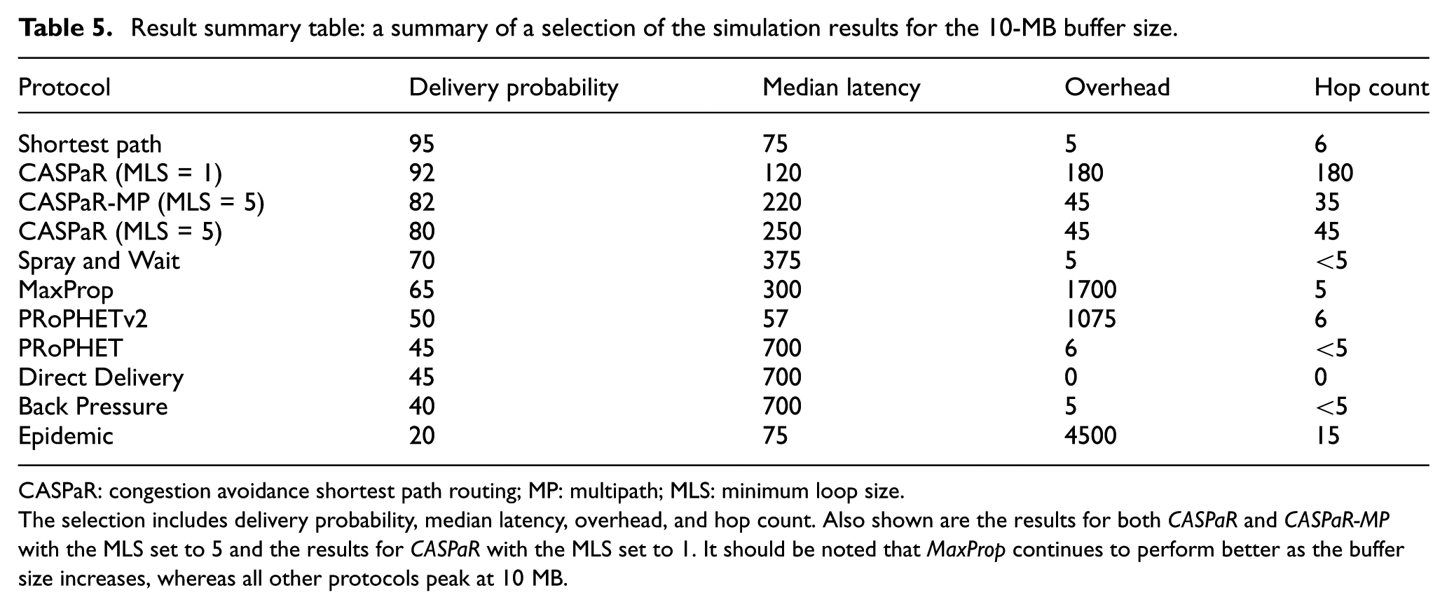
CASPaR: congestion avoidance shortest path routing; MP: multipath; MLS: minimum loop size.

The selection includes delivery probability, median latency, overhead, and hop count. Also shown are the results for both CASPaR and CASPaR-MP with the MLS set to 5 and the results for CASPaR with the MLS set to 1. It should be noted that MaxProp continues to perform better as the buffer size increases, whereas all other protocols peak at 10 MB.

Conclusion

We have developed an extensible protocol, one that does not depend on mobility predictions or data mules. A protocol that can handle a heavy network load using small network resources and by all measurements is one that can handle an even heavier network load than tested here. We have shown that CASPaR improves network performance where Spray and Wait and MaxProp, while also performing well under the same experimental conditions, require much larger buffers and in the case of MaxProp a much larger overhead to do so. It is clear that a multi-path approach to costing routes from source to destination is beneficial as CASPaR-MP outperformed CASPaR. It is also apparent that routing, at least when applied to the network model tested here, is a viable option and should be further explored.

Future work

Several avenues can be explored in continuing work with CASPaR. First, various simulation parameters should be applied to more extensively test CASPaR. Varying the network model to see how CASPaR performs in various scenarios is interesting. Also, testing a random routing protocol and comparing its results with the results shown here is important. Second, the CASPaR-MP variation outperformed CASPaR and should be further explored. The next logical step along the CASPaR-MP algorithm is to experiment with breaking packets at the source and rebuilding them at the destination and whether or not this provides any performance increase. This may have to be performed as a function of an increased network load in order to see any benefit. Third, an obvious question arises from studying the latency in Figure 7 which is “How do we move packets from high- to low-latency bins?” The answer might be some hybrid protocol, a combination of two or more protocols that excel in specific topologies. Combining parts of CASPaR, MaxProp, and Spray and Wait might yield some interesting results. Fourth, determine how CASPaR-MP and Shortest Path perform at even higher network loads. Is there a point at which CASPaR-MP approaches or even surpasses the performance of Shortest Path?

Footnotes

Handling Editor: Hongke Zhang

Declaration of conflicting interests

The author(s) declared no potential conflicts of interest with respect to the research, authorship, and/or publication of this article.

Funding

The author(s) received no financial support for the research, authorship, and/or publication of this article.

References

Perkins

Royer

Ad-hoc on-demand distance vector routing. In: Second IEEE workshop on mobile computing systems and applications, Washington, DC, 25–29 February 1999, pp.90–100. New York: IEEE.

Jacquet

Muhlethaler

Clausen

et al . Optimized link state routing protocol for ad hoc networks. In: IEEE international multi topic conference, Lahore, Pakistan, 30 December 2001, pp.62–68. New York: IEEE.

Haas

Pearlman

Samar

. The zone routing protocol (ZRP) for ad hoc networks [Draft]. IETF, https://tools.ietf.org/html/draft-ietf-manet-zone-zrp-04 (2002).

D’Souza

Jose

Routing approaches in delay tolerant networks: a survey. Int J Comput Appl 2010; 1(17): 8–14.

Vahdat

Becker

Epidemic routing for partially-connected ad hoc networks. Technical report, Duke University, Durham, NC, April 2000.

Lindgren

Doria

Scheln

Probabilistic routing in intermittently connected networks. SIGMOBILE Mob Comput Commun Rev 2003; 7(3): 19–20.

Naziruddin

Pushpalatha

A dynamic approach to history based DTN routing on delivery predictabilities. Int J Appl Eng Res 2015; 10(7): 17275–17282.

Burgess

Gallagher

Jensen

. MaxProp: routing for vehicle-based disruption-tolerant networks. In: 25th IEEE international conference on computer communications, Barcelona, 23–29 April 2006, pp.1–11. New York: IEEE.

Spyropoulos

Psounis

Raghavendra

. Spray and wait: an efficient routing scheme for intermittently connected mobile networks. In: SIGCOMM workshop on delay-tolerant networking, Philadelphia, PA, 26 August 2005, pp.252–259. New York: ACM.

10.

Moeller

Sridharan

Krishnamachari

et al . Routing without routes: the backpressure collection protocol. In: 9th international conference on information processing in sensor networks, Stockholm, 12–16 April 2010, pp.279–290. New York: ACM.

11.

Dvir

Vasilakos

. Backpressure-based routing protocol for DTNs. In: SIGCOMM 2010 conference, New Delhi, India, 30 August–3 September 2010, pp.405–406. New York: ACM.

12.

Ryu

Ying

Shakkottai

. Back-pressure routing for intermittently connected networks. In: IEEE INFOCOM, San Diego, CA, 14–19 March 2010, pp.1–5. New York: IEEE.

13.

Alresaini

Sathiamoorthy

Krishnamachari

et al . Backpressure with adaptive redundancy (BWAR). In: 2012 IEEE, INFOCOM, Orlando, FL, 25–30 March 2012, pp.2300–2308. New York: IEEE.

14.

Hui

Crowcroft

Yoneki

BUBBLE rap: social-based forwarding in delay-tolerant networks. IEEE T Mobile Comput 2011; 10(11): 1576–1589.

15.

Caini

Cruickshank

Farrell

et al . Delay- and disruption-tolerant networking (DTN): an alternative solution for future satellite networking applications. Proc IEEE 2011; 99(11): 1980–1997.

16.

Stewart

Kannan

Dvir

et al . CASPaR: congestion avoidance shortest path routing for delay tolerant networks. In: 2016 international conference on computing, networking and communications, Kauai, HI, 15–18 February 2016, pp.1–5. New York: IEEE.

17.

Ellens

Spieksma

Mieghem

et al . Effective graph resistance. Linear Algebra Appl 2011; 435(10): 2491–2506.

18.

Silva

Burleigh

Hirata

et al . A survey on congestion control for delay and disruption tolerant networks. Ad Hoc Netw 2015; 25(1): 480–494.

19.

Keränen

Ott

Kärkkäinen

. The ONE simulator for DTN protocol evaluation. In: International conference on simulation tools and techniques, Rome, 2–6 March 2009, pp.1–10. New York: Springer.

20.

Wang

Lin

et al . Probabilistic routing based on two-hop information in delay/disruption tolerant networks. J Electr Comput Eng 2015; 2015: 9.

21.

Han

Chung

YW.

An improved PRoPHET routing protocol in delay tolerant network. Sci World J 2015; 2015: 623090.

22.

Kim

Nam

Choi

et al . Probability-based spray and wait protocol in delay tolerant networks. In: The international conference on information networking, Phuket, Thailand, 10–12 February 2014, pp.412–416. New York: IEEE.

23.

You

et al . Dynamic groups based adaptive DTN routing algorithms in social networks. Int J Distrib Sens N 2014; 10(4): 245369.

24.

Zhang

Jin

. Dynamic spray and wait routing protocol for delay tolerant networks. In: Park

Zomaya

Yeo

et al . (eds) Network and parallel computing. Berlin, Heidelberg: Springer, 2012, pp.69–76.

25.

Pathak

Gondaliya

Raja

. A survey on PROPHET based routing protocol in delay tolerant network. In: 2017 international conference on emerging trends and innovation in ICT, Pune, India, 3–5 February 2017, pp.1–7. New York: IEEE.

26.

Desta

Hyyti ä

Ker ä nen

et al . Evaluating (Geo) content sharing with the ONE simulator. In: International symposium on mobility management and wireless access, Barcelona, 3–8 November 2013, pp.37–40. New York: ACM.

27.

Wolf

et al . A named data approach for DTN routing. In: 2017 wireless days, Porto, 29–31 March 2017, pp.163–166. New York: IEEE.

28.

Dhurandher

Borah

Woungang

et al . Advances on broad-band wireless computing, communication and applications. In: 11th international conference on broad-band wireless computing, communication and applications, Asan, South Korea, 5–7 November 2017, pp.491–499. New York: Springer.

29.

Mangrulkar

Atique

. Performance evaluation of flooding based delay tolerant routing protocols. In: National conference on emerging trends in computer science and information technology, Punjab, India, 4–5 March 2011, pp.35–40. New York: IEEE.

30.

Grasic

Davies