Sage Journals: Discover world-class research

Abstract

We propose a dynamic energy balanced max flow routing algorithm to maximize load flow within the network lifetime and balance energy consumption to prolong the network lifetime in an energy-harvesting wireless sensor network. The proposed routing algorithm updates the transmission capacity between two nodes based on the residual energy of the nodes, which changes over time. Hence, the harvested energy is included in calculation of the maximum flow. Because the flow distribution of the Ford–Fulkerson algorithm is not balanced, the energy consumption among the nodes is not balanced, which limits the lifetime of the network. The proposed routing algorithm selects the node with the maximum residual energy as the next hop and updates the edge capacity when the flow of any edge is not sufficient for the next delivery, to balance energy consumption among nodes and prolong the lifetime of the network. Simulation results revealed that the proposed routing algorithm has advantages over the Ford–Fulkerson algorithm and the dynamic max flow algorithm with respect to extending the load flow and the lifetime of the network in a regular network, a small-world network, and a scale-free network.

Keywords

Dynamic maximum flow routing algorithm load flow energy-harvesting wireless sensor network energy balanced

Introduction

Nodes of traditional wireless senor networks (WSNs) are typically powered by batteries. Once the energy is depleted, the node is “dead,” so the lifetime of a network is limited to its battery capacity. Moreover, it is very difficult and costly to replace batteries due to the deployment of nodes in difficult-to-access environments or large numbers of nodes.¹ As a result, the limited lifetime of the network creates a bottleneck in WSNs. Energy-aware routing is one of the main approaches for balancing energy consumption and prolonging network life. Along with the development of hardware technology, it is possible for nodes to harvest energy from the ambient environment, such as from radio frequency,² solar,³ thermal,⁴ and vibrations.⁵ The emergence of energy-harvesting technology partly alleviates the problem with the energy constraint of the nodes and makes self-powering, long-lasting energy-harvesting wireless sensor networks (EHWSNs) possible.

With the introduction of energy harvesting, the objective of routing algorithm for EHWSNs is maximizing the network’s workload since energy can be replenished. Bogliolo et al.⁶ first proposed the maximum energetically sustainable workload (MESW) problem and showed that the EHWSN can be cast into an instance of a modified max flow problem. The article also gives the reachable upper bound for the workload that can be sustained by the network. To achieve the max workload, the data rate and the energy-harvesting rate must satisfy a definite constraint. Then, Lattanzi et al.⁷ proposed a methodology that made use of graph algorithms and network simulations for evaluating the MESW starting from a network topology, a routing algorithm, and a distribution of the environmental power available at each node. The main challenge for routing algorithm in EHWSN is that the energy harvesting strongly depends on the environment power conditions, which changes over time. Seraghiti and Bogliolo⁸ presented a theoretically optimum max flow routing algorithm that makes EHWSNs able to transparently adapt to time-varying environmental power conditions during their normal operation. Bogliolo et al.⁹ proposed a self-adapting maximum flow (SAMF) routing strategy which was able to route any sustainable workload while automatically adapting to time-varying operating conditions. Wu et al.¹⁰ proposed a centralized power efficient routing algorithm energy-harvesting genetic-based unequal clustering-optimal adaptive performance routing algorithm (EHGUC-OAPR) to balance the network energy and improve delivery ratio. The objective of these studies focuses on the optimal routing to adapt the variation of environment conditions for maintaining the network energy sustainable. Due to the unstable environment conditions, the harvested energy may be not enough to sustain the network in many cases. In view of the max flow and network lifetime when the network is not energy sustainable, an energy balanced dynamic maximum flow (EB-DMF) routing algorithm is proposed in this article. The proposed routing algorithm has two features that distinguish it from the Ford–Fulkerson (FF) algorithm:

Nodes of the network can harvest energy from their environment, so the energy of the nodes is variable. The static FF algorithm calculates the capacity based on the initial energy of nodes, with the result that the harvested energy cannot be included in the capacity. The load flow of the network is restricted to the initial energy of nodes. To remove this constraint, the capacity of the edge is updated according to its residual energy when the flow of the residual network is not sufficient for the next delivery. The improved algorithm is defined as a dynamic max flow (DMF) routing algorithm.

The FF algorithm randomly and disproportionately allocates the flow on the augmenting path, causing unbalanced energy consumption among nodes. The more flow the augmenting path carries, the more energy the nodes on it will consume. To balance the flow distribution, the capacity of the edges is updated when the flow of any edge is not sufficient for the next delivery. To balance energy consumption and prolong network life, the node chooses the next layer neighbor (NLN) with maximum residual energy as its next hop.

Simulations were conducted to perform a comparative study by applying FF, DMF, and EB-DMF algorithms to three different network models, to verify the validity of the EB-DMF algorithm. The network models are a uniform distribution network model, the Watts–Strogatz (WS) model,¹¹ and the Barabasi–Albert (BA) model.¹² By comparing the FF, DMF, and EB-DMF algorithms to various network models, we can obtain a deep understanding of the performance of EB-DMF in real EHWSN applications. The simulation results will help guide EB-DMF engineering practice in EHWSN, incorporating issues such as network deployment, routing configuration, and application range.

The remainder of this article is organized as follows. Section “Related work” presents a review of relevant prior work. The “Network environment and problem” section explains the network environment of the proposed algorithm and describes the problem. The proposed routing algorithm is described in “Routing algorithm”. Section “Simulation” discusses the simulation results. Finally, the article is concluded in section “Conclusion and future works.”

Related works

Because of the character of energy harvesting, most existing routing algorithms are not suitable for EHWSN. EHWSN has scale-free and small-world properties, and it is necessary to study the routing process according to the particular requirements of these types of networks. Accordingly, in this section, we describe related research progress in two ways: routing in EHWSN and complex networks.

Routing in EHWSN

There are typically two types of EHWSN:¹³ the first is still powered by batteries, but the energy of the batteries can by supplied by energy harvesting, while the second type is powered only by harvested energy. Accordingly, the routing algorithms can be divided into two classes. For the first type of EHWSN, the routing design always aims to improve energy efficiency and prolong network life. Voigt et al.¹⁴ first proposed solar-aware routing that preferentially routes traffic via nodes powered by solar energy to save battery energy. sLEACH routing was also developed to extend the lifetime of the network.¹⁵ Islam et al.¹⁶ proposed A-sLEACH, an extension of sLEACH. For the second type of EHWSN, the objective of most routing is to maximize the throughput and data delivery ratio of the network under the condition that the network is energetic sustainability. In Meng et al.,¹³ an adaptive energy-harvesting aware clustering (AEHAC) routing protocol for EHWSNs was proposed to maintain available nodes and improve the network throughput. In Eu and Tan,¹⁷ a routing method that included the network deploying environment was proposed to increase the throughput of the network.

Routing in complex networks

Large complex communication networks, such as the network society,¹⁸ the World Wide Web,¹⁹ and WSNs²⁰ have drawn significant attention. Many routing strategies have been proposed for WSNs to improve the transmission capacity of networks and avoid congestion based on complex network theory, including efficient routing, optimal routing, local routing, and hub avoidance strategies.^21–27

To verify the performance of EB-DMF, we applied the proposed algorithm to a complex network.

Network environment and problem formulation

Network environment

Given an EHWSN as shown in Figure 1, this article assumes that all data packets are generated by the source sensors and are transmitted to the sink sensor by the router in a multi-hop manner by applying the routing strategy. All sensors are assumed to have the same energy-harvesting rate and all the source sensors are assumed to have the same data packets rate.⁶ Moreover, all nodes have the same battery capacity $C$ . All sensors execute the sensing task and then periodically send the data packets to the sink senor in every time period $t_{0}$ . Therefore, the sink node can acquire the energy information about all sensors and the topology of the network by the periodic communication (Figure 2).

Figure 1.

An energy-harvesting wireless sensor network.

Figure 2.

The equivalent model of the EHWSN.

In this article, the max flow algorithm is applied to determine the routing strategy which maximized the load flow and lifetime of the network. This article assumes that all the source sensors are connected to the virtual source node $n_{S}$ and all the sink sensors are connected to the virtual sink node $n_{D}$ . Therefore, the virtual nodes have infinite energy. The energy of the real sensors is limited to the capacity of the battery. Consider a network with $M$ router sensors, let $N = {n_{i} | 1 \leq i \leq M}$ denote the sets of all router sensors. The virtual source node sends the data packets in every time period $τ$ . During the period, the packets are routed from the virtual source node to the virtual sink node. Let $r = {n_{S}, n_{i}, \dots, n_{D}}$ denote the routing path. Taking Figure 3 for example, the routing path can be expressed as ${n_{s}, n_{2}, n_{4}, n_{D}}$ .

Figure 3.

The example of routing path in EHWSN.

To obtain minimum hop end-to-end communication, we first adopt the breadth-first searching (BFS) algorithm to obtain hierarchical information on the network. The BFS begins at the source node and searches all neighboring nodes. Then, based on those neighbor nodes in turn, unvisited neighbor nodes are searched, and so on. After BFS, the neighbors of node $n_{i}$ can be divided into three types: upper-layer neighbors (ULNs), NLNs, and same-layer neighbors (SLN). ULNs are neighbors toward the source node and NLNs are neighbors toward the destination. Neighbors situated at the same layer of $n_{i}$ are SLNs. The ULN set of $n_{i}$ is defined as $U_{i}$ , the SLN set of $n_{i}$ is defined as $S_{i}$ , and the NLN set of $n_{i}$ is defined as $N_{i}$ . In Figure 3, nodes 1–3 belong to layer 1 and nodes 4–6 belong to layer 2. Taking node 5 as an example, $U_{5} = {n_{1}, n_{2}, n_{3}}$ , $S_{5} = {n_{4}, n_{5}, n_{6}}$ .

The virtual source node sends $p$ packets in every time period $t_{0}$ . Then, the packets are forwarded by the routers. During this process, the nodes consume energy. Meanwhile, the nodes also harvest energy. The energy consumption of the nodes includes two parts: data processing and data transmission. Experimental measures have shown that data transmission generally consumes more energy than data processing.²⁸ Thus, we can take the consumption of data transmission as the energy consumption of the node, ignoring data processing consumption. Let $E_{r}$ denote the energy consumption of the node when the node receives one packet, and $E_{s}$ denote the energy consumption of the node when the node transmits one packet. The harvested energy of the nodes during 1 s is denoted as $E_{h}$ . Let $E_{i} (t)$ denote the residual energy of node $n_{i}$ at time $t$ . The time $T$ is called the lifetime of the network when the first failure node (the energy of the node is exhausted) appears, if $E_{i} (t) = 0$ holds, where $\forall n_{i} \in N$ . The residual energy determines the ability of the nodes to forward packets. Let $C_{i} (t)$ define the packets that can be forwarded by node $n_{i}$ at time $t$ .

In this article, the proposed routing algorithm dynamically calls the max flow algorithm. Assume that the interval of calling the max flow algorithm is

{T_{1}, T_{2}, \dots, T_{k}}

(1)

Then, the time of calling the max flow algorithm for $k$ times can be described as, called the update time

t_{k} = {\begin{matrix} \sum_{m = 1}^{k - 1} T_{m}, k > 1 \\ 0, k = 1 \end{matrix}

(2)

Let $C_{ij} (t_{k})$ denote the packets that can be transmitted by the communication link between node $n_{i}$ and node $n_{j}$ at time $t_{k}$ , which is called the edge capacity. The communication link between node $n_{i}$ and node $n_{j}$ is called the edge, noted as $(n_{i}, n_{j})$ . Let $f_{ij} (t_{k})$ denote the packets transmitted by $(n_{i}, n_{j})$ that is calculated by max flow algorithm at time $t_{k}$ , which is called the edge flow. Let $f (t_{k})$ denote the packets transmitted by the network that is calculated by max flow algorithm at time $t_{k}$ . Let $r_{m}^{k}$ denote the routing path (or augmenting path) that is calculated by max flow algorithm at time $t_{k}$ .

The set of routing paths can be defined as $R^{k}$

R^{k} = {r_{1}^{k}, r_{2}^{k}, \dots, r_{m}^{k}}

(3)

The flow of augmenting path $r_{m}^{k}$ is defined as $f_{m}^{k}$ .

Let $F$ denote the packets that the network can transmit in its lifetime, called the load flow.

Problem formulation

The main work of this article is to design a routing-based on max flow algorithm for EHWSN to extend the load flow and the lifetime of the network.

The network of the lifetime can be described as

E_{i} (T) = 0, \forall n_{i} \in N

(4)

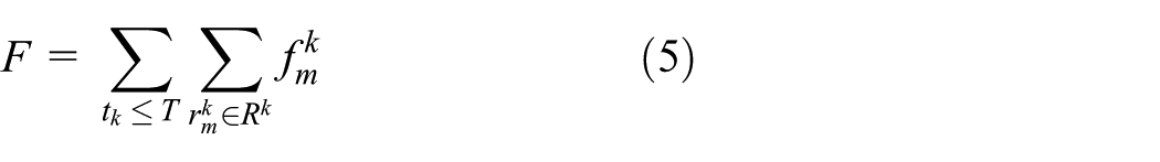
The load flow of the network is the flow sum of all the routing paths within the network lifetime, which can be described as

F = \sum_{t_{k} \leq T} \sum_{r_{m}^{k} \in R^{k}} f_{m}^{k}

(5)

As shown in objective Function (6), this article aims at maximizing lifetime and the max flow while satisfying Constraints (7)–(19)

Maximize {T, F}

(6)

The source node sends $p$ number of packets along one augmenting path in 1 s. The routings found during $τ$ are $R_{τ} = {r_{t + 1}, r_{t + 2}, \dots, r_{k}, \dots, r_{t + τ}}$ , the elements in $r_{τ}$ can be identical, and $r_{τ} \in P$ . $fla g_{i} (k)$ indicates whether $n_{i}$ is included in $r_{k}$

fla g_{i} (k) = {\begin{matrix} 1, if n_{i} \in r_{k} \\ 0, if n_{i} \notin r_{k} \end{matrix}

(7)

The counts of $R_{τ}$ passing through $n_{i}$ during time $τ$ can be expressed as

coun t_{i} (τ) = \sum_{r_{k} ε R_{τ}} fla g_{i} (k)

(8)

Suppose the residual energy of node $n_{i}$ at time $t$ is $E_{i} (t)$ , the harvested energy of the node during 1 s is $E_{h}$ , and the energy-harvesting rate of all nodes is the same. The residual energy of $n_{i}$ at time $t + τ$ can be calculated as

E_{i} (t + τ) = E_{i} (t) + E_{h} * τ - (E_{r} + E_{s}) * coun t_{i} (τ) p

(9)

All nodes have the same initial energy, which is equal to the battery capacities C, the above formula can be expressed as

E_{i} (τ) = C + E_{h} * τ - (E_{r} + E_{s}) * coun t_{i} (τ) p

(10)

The energy of the nodes is limited to the battery capacity

E_{i} (t) \leq C

(11)

For max flow algorithm, the flow of the augmenting path is determined by the minimum edge capacity

f_{m}^{k} = min (C_{ij} (t_{k})), n_{i} \in r_{m}^{k} and n_{j} \in r_{m}^{k}

(12)

The edge capacity is determined by the energy of the nodes

C_{i} (t_{k}) = \frac{E_{i} (t_{k})}{E_{r} + E_{s}}

(13)

The virtual nodes have infinite energy. The edge capacities between them and their neighbors are determined by the nodes connected to them: if node $n_{i}$ is connected to the source node, the edge capacity between $n_{S}$ and $n_{i}$ can be expressed as

C_{Si} (t_{k}) = C_{i} (t_{k})

(14)

In a similar way, if node $n_{j}$ is connected to the destination node, we obtain

C_{jD} (t_{k}) = C_{j} (t_{k})

(15)

For other nodes, we can calculate the edge capacity $C_{ij} (t)$ as follows

C_{ij} (t_{k}) = α_{ij} (t_{k}) * C_{i} (t_{k})

(16)

The edge capacity can be distributed based on $C_{i} (t_{k})$ . The distribution ratio of the edge capacity is defined as $α_{ij} (t_{k})$ and calculated based on the energy of its NLN or SLN. Here, the nodes are restricted to communicate with their NLN when they have NLN to achieve minimum hop end-to-end communication. Unless the nodes have no NLN, they communicate with their SLN. The factor ${α_{i}}_{j} (t_{k})$ is calculated as

α_{ij} (t_{k}) = {\begin{matrix} \frac{E_{j} (t_{k})}{\sum_{n_{j} \in N_{i}} E_{j} (t_{k})}, if N_{i} \notin \emptyset \\ \frac{E_{j} (t_{k})}{\sum_{n_{j} \in S_{i}} E_{j} (t_{k})}, if N_{i} = \emptyset \end{matrix}

(17)

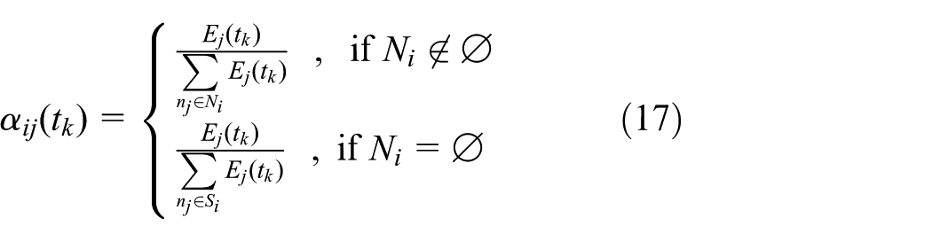
Applying formulas (13) and (17) to formula (16)

C_{ij} (t_{k}) = {\begin{matrix} \frac{E_{j} (t_{k})}{\sum_{n_{j} \in N_{i}} E_{j} (t_{k})} * \frac{E_{i} (t_{k})}{E_{r} + E_{s}}, if N_{i} \notin \emptyset \\ \frac{E_{j} (t_{k})}{\sum_{n_{j} \in S_{i}} E_{j} (t_{k})} * \frac{E_{i} (t_{k})}{E_{r} + E_{s}}, if N_{i} = \emptyset \end{matrix}

(18)

The packets transmitted by $(n_{i}, n_{j})$ should less than the edge capacity

f_{ij} (t_{k}) \leq C_{ij} (t_{k})

(19)

The more packets the node transmitted, the node tends to deplete its energy, and the network is easy to die. Meanwhile, the value of $f_{m}^{k}$ is small. Therefore, the routing strategy balanced the energy consumption among the nodes can extend the lifetime and load flow of the network.

Routing algorithm

In this section, we use a simple routing example to illustrate the proposed EB-DMF algorithm, and then explain how this realizes dynamic energy balanced routing. We finally provide a flow chart for DMF and EB-DMF. Before describing the workings of EB-DMF in detail, the objectives of EB-DMF are stated explicitly:

Minimum hop end-to-end communication to fulfill short latency communication requirements.

Dynamically updating the capacity to achieve larger flow load.

Balanced energy consumption to increase overall network lifetime.

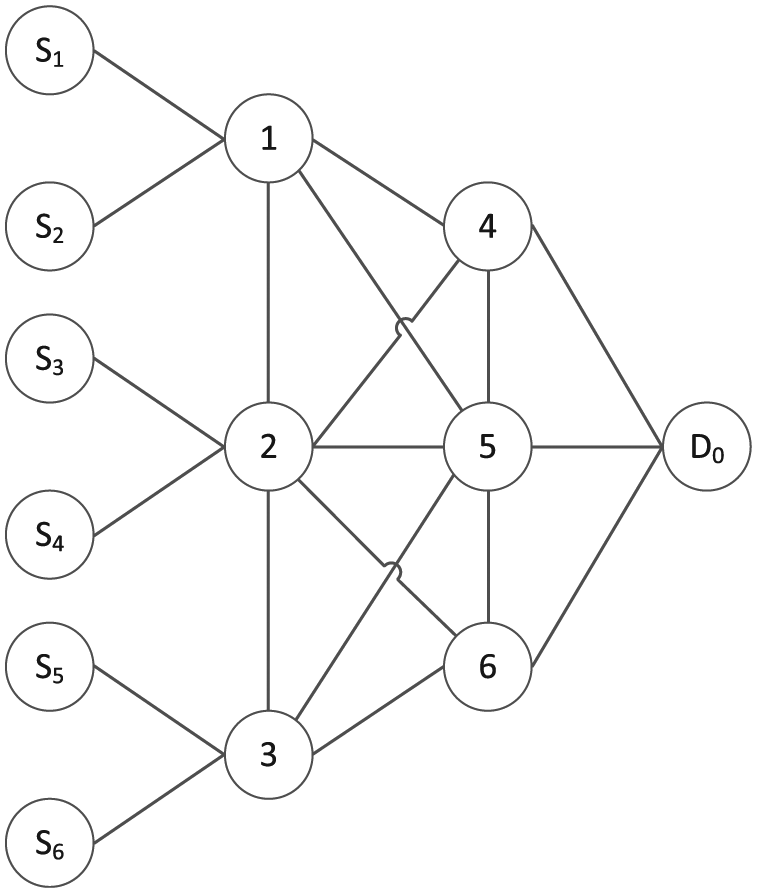
To explain the problem clearly, we consider the example of a regular network topology, as shown in Figure 4. This is a small network of six nodes, one virtual source node, and one virtual destination node. Assuming that all source nodes are connected to the virtual source node and all destination nodes are connected to the virtual destination nodes, all the virtual nodes have infinite energy.⁷

Figure 4.

An example of EHWSN topology.

FF algorithm

The FF algorithm can be introduced to maximize the flow load of the network under the circumstance that the energy of nodes is constrained. The initial energy of all nodes except source and destination nodes is 0.27J, and $E_{r} = 0.001 J, E_{s} = 0.0005 J$ . The edge capacity of FF can be calculated according to formula (18). The edge capacities of Figure 4 are shown in Figure 5. Here, we only consider a packet sent from a source node to a destination node in a directed network because the process of delivering packets is revisable.

Figure 5.

The edge capacity of the network.

The flow of edge $(n_{i}, n_{j})$ is defined as $f (n_{i}, n_{j})$ , which presents the sum of the flow on the found augmenting paths across $(n_{i}, n_{j})$ .

The residual flow of $(n_{i}, n_{j})$ is defined as $r (n_{i}, n_{j})$ , which represents the containable flow allowed by $(n_{i}, n_{j})$

r (n_{i}, n_{j}) = C_{ij} (t_{1}) - f (n_{i}, n_{j})

(20)

The process of looking for an augmenting path and its flow using the FF algorithm is described as follows.

Look for augmenting path $r_{k}^{1}$ and record the flow $f_{k}^{1}$ of the augmenting path.

Add $f_{p_{k}}$ to the flow of all edges on $r_{k}^{1}$ $f (n_{i}, n_{j}) = f (n_{i}, n_{j}) + f_{k}^{1}, if (n_{i}, n_{j}) \in r_{k}^{1}$ .

After applying this algorithm to Figure 5, the augmenting paths and flow are as given in Table 1.

Table 1.

Routing path and flow (sorted by finding order at $t = 0$ ).

Routing path	Flow
${r_{1}}^{1} {n_{S}, n_{1}, n_{4}, n_{D}}$	${f_{1}}^{1} = 300$
${r_{2}}^{1} {n_{S}, n_{1}, n_{5}, n_{D}}$	$f_{2}^{1} = 300$
${r_{3}}^{1} {n_{S}, n_{2}, n_{4}, n_{D}}$	$f_{3}^{1} = 200$
${r_{4}}^{1} {n_{S}, n_{2}, n_{5}, n_{D}}$	$f_{4}^{1} = 200$
${r_{5}}^{1} {n_{S}, n_{2}, n_{6}, n_{D}}$	$f_{5}^{1} = 200$
${r_{6}}^{1} {n_{S}, n_{3}, n_{5}, n_{D}}$	$f_{6}^{1} = 100$
${r_{7}}^{1} {n_{S}, n_{3}, n_{6}, n_{D}}$	$f_{7}^{1} = 300$

The max flow of the network is

f (t_{1}) = \sum_{m = 1}^{9} f_{m}^{1} = 1600

(21)

The order of augmenting paths is irrelevant because the order does not affect the final value of $f (n_{i}, n_{j})$ and $f$ when the algorithm stops. $f (n_{i}, n_{j})$ represents the sum of the flow on the found augmenting paths across $(n_{i}, n_{j})$ , so the value of $f (n_{i}, n_{j})$ may vary due to the different order of found augmenting paths during the execution of the program, but the value of $f (n_{i}, n_{j})$ is constant regardless of the finding order when the algorithm stops. Similarly, the value of $f (t_{1})$ is constant regardless of the finding order when the algorithm stops. Thus, the flow of all edges can be described as shown in Figure 6.

Figure 6.

The flow of all edges after FF.

DMF routing algorithm

The battery is not the only power source in EHWSN. The FF algorithm only considers the battery energy of the node, regardless of the energy harvested by the node from the ambient environment. We propose a DMF routing algorithm to solve this problem; in DMF, the edge capacity is updated according to the residual energy of the node. The process of finding augmenting paths will not be restated, and this is described in section FF algorithm. If we enter all edge capacities $C_{ij} (t_{k})$ and the topology $G$ into the FF algorithm, we can obtain the flow of all edges $f_{ij} (t_{k})$ and the max flow $f (t_{k})$ . Only the output of the FF algorithm is used to consider the flow change during packet delivery.

The edge capacities can be calculated according to formulas (14)–(18). After updating the edge capacities, we can use FF to calculate the flow of all edges $f_{ij} (t_{k})$ and the max flow $f (t_{k})$ , the flow of the edges is shown in Figure 6.

We define the residual flow of the network as $f_{r} (t)$ to denote the flow that can be sustained at time $t$

f_{r} (t) = f (t_{k}) - p * (t - t_{k}), if t_{k} \leq t \leq t_{k + 1}

(22)

Formula (22) shows the residual flow of the network at time $t$ , equal to the max flow calculated based on the previous edge capacities updating time with the number of delivered packets during the period subtracted.

The edge capacity is updated when the residual flow of the network is less than $p$ , which means the network cannot support the next delivery. Thus, we update the edge capacities when (Algorithm 1)

f_{r} (t) \leq p

(23)

Here, $fla g_{ij} (k)$ is defined to indicate whether edge $(n_{i}, n_{j})$ is included in $r_{k}$

fla g_{ij} (k) = {\begin{matrix} 1, if (n_{i}, n_{j}) \in r_{k} \\ 0, if (n_{i}, n_{j}) \notin r_{k} \end{matrix}

(24)

Algorithm 1.

DMF routing algorithm.

The counts of $R_{τ}$ passing through edge $(n_{i}, n_{j})$ during time $τ$ can be expressed as

coun t_{ij} (τ) = \sum_{r_{k} \in R_{τ}} fla g_{ij} (k)

(25)

The residual flow of edge $(n_{i}, n_{j})$ at time $t$ is defined as $f_{r (n_{i}, n_{j})} (t)$

f_{r (n_{i}, n_{j})} (t) = f_{ij} (t_{k}) - p * coun t_{i} (t - t_{k}), if t_{k} \leq t < t_{k + 1}

(26)

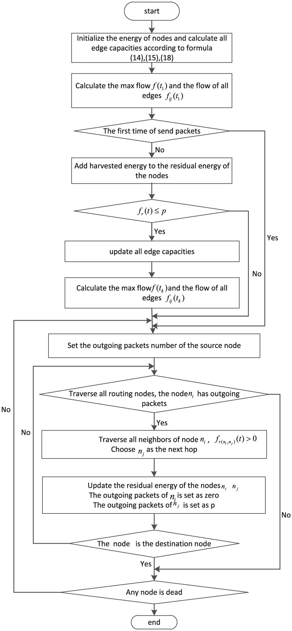
The DMF algorithm can be described as follows:

Initialize the energy of nodes, and calculate all edge capacities, then calculate the flow of all edges $f_{ij} (t_{k})$ and max flow $f (t_{k})$ .

If it is the first instance of packet sending, the residual energy of the nodes does not need to be updated because the nodes have not yet harvested energy. Otherwise, update the residual energy of the nodes, then decide whether to update edge capacities according to formula (23); if the edge capacities are updated, we need to recalculate the flow of all edges $f_{ij} (t_{k})$ and the max flow $f (t_{k})$ based on FF.

Set the outgoing packet number of the source node as $p$ .

If the residual flow of edge $(n_{i}, n_{j})$ is not equal to zero, which means the edge can support packet forwarding in this interval, then we choose $n_{j}$ as the next hop.

When $n_{j}$ is $n_{D}$ , which means the delivery is over in this interval, we need to judge whether any node is dead. If one node dies, the life of the network ends. Otherwise, the next delivery should be executed. Jump to step (3). When $n_{j}$ is not $n_{D}$ , we still need to find the next hop for $n_{i}$ . Jump to step (4).

To explain the process of routing packets and describe the update time, we can apply the DMF algorithm to an example (shown in Figure 5). Step 1 has been discussed in section FF algorithm, and the FF algorithm will not be restated here. The output of the FF algorithm (as shown in Figure 6) is used to represent the process. Assume that the source node sends the first packet at $t = 0$ and sends 20 packets per second, and that the packet sending interval is 1 s. According to Table 1, the flow of the network is 1600, $t_{s}$ denotes the start time, $t_{e}$ denotes the end time, and $Δ t = t_{e} - t_{s}$ . $Δ f = p . Δ t$ denotes the flow of the network during $Δ t$ ; $f_{r} (t)$ denotes the residual flow of the network, which can be calculated using formula (22). The routing process is described in Table 2.

Table 2.

The routing process.

$t_{s} (s)$	$t_{e} (s)$	R	$Δ f$	$f_{r} (t)$
0	15	${n_{S}, n_{1}, n_{4}, n_{D}}$	$15 \times 20 = 300$	1300
15	30	${n_{S}, n_{1}, n_{5}, n_{D}}$	$15 \times 20 = 300$	1000
30	40	${n_{S}, n_{2}, n_{4}, n_{D}}$	$10 \times 20 = 200$	800
40	50	${n_{S}, n_{2}, n_{5}, n_{D}}$	$10 \times 20 = 200$	600
50	60	${n_{S}, n_{2}, n_{6}, n_{D}}$	$10 \times 20 = 200$	400
60	65	${n_{S}, n_{3}, n_{5}, n_{D}}$	$5 \times 20 = 100$	300
65	79	${n_{S}, n_{3}, n_{6}, n_{D}}$	$14 \times 20 = 280$	20
79	–	Updating edge capacities

The augmenting path $r_{k}^{1}$ is as shown in Table 1; for the FF routing algorithm, this stops at $t = 79$ because the residual flow of the network cannot support delivery of the next packet. For the DMF routing algorithm, when the residual load flow of the network cannot support the next packet delivery, edge capacities are updated and this process repeated until the flow of the network calculated by FF is less than $p$ . Thus, the DMF routing algorithm can extend the load flow compared with the FF routing algorithm.

Energy balanced dynamic max flow routing algorithm

Due to the unbalanced distribution of the edge flow, the energy consumption of nodes is not balanced and the network will terminate early. Taking Figure 6 as an example, although nodes 1, 2, and 3 have the same energy, the flow distribution calculated from the maximum flow is not balanced. The flow of edge $(n_{s}, n_{3})$ is less than the flow of edge $(n_{s}, n_{1})$ , which results in node 3 consuming less energy compared to nodes 1 and 2. Similarly, node 5 consumes more energy than nodes 4 and 6. Therefore, we propose the EB-DMF routing algorithm to improve the DMF routing algorithm. To achieve this goal, the neighbor node with maximum residual energy is chosen as the next hop, and the update time of DMF is changed. The residual flow of edge and network lifetime is compared. According to the routing mechanism discussed previously, which means energy consumption within the same layer is balanced, if the residual flow of one edge is less than $p$ , which means the flow of the edge calculated by FF is less than that of other edges, the energy consumption may not be balanced during next delivery. Thus, we update the edge capacities when (Algorithm 2)

f_{r (n_{i}, n_{j})} \leq p

(27)

Algorithm 2.

EB-DMF routing algorithm.

The flow chart of the EB-DMF routing algorithm is shown as Algorithm 2.

Based on the example shown in Figure 5, the routing process can be described as follows:

From $t = 1$ to $t = 2$ , the packets are transmitted along augmenting path $r_{1}^{1} {n_{s}, n_{1}, n_{4}, n_{D}}$ , and from $t = 2$ to $t = 3$ , the packets are transmitted along augmenting path $r_{2}^{1} {n_{s}, n_{2}, n_{5}, n_{D}}$ . The EB-DMF routing algorithm chooses the next hop based on the residual energy of the nodes. Thus, the source node chooses node 2 as its next hop instead of node 1 because node 1 has consumed energy during the last delivery, and the residual energy of node 1 is less than node 2, which is similar to node 5.

From $t = 3$ to $t = 4$ , the packets are transmitted along augmenting path $r_{3}^{1} {n_{S}, n_{3}, n_{6}, n_{D}}$ .

The delivery of packets repeats the above process in the order ${r_{1}^{1}, r_{2}^{1}, r_{3}^{1}}$ until the residual energy of one edge is less than or equal to $p = 20$ , then the edge capacities and the flow of the network are recalculated. This happens at $t = 26$ , and the residual flow of all edges is shown in Figure 7.

Figure 7.

The residual flow of all edges at $t = 26$ .

From Figure 7, we can see that the residual flow of $(n_{2}, n_{5})$ is less than 20; therefore, the edge capacities need to be updated.

The second update is at $t = 66$ , and here the residual flow of all edges is shown in Figure 8. From Figure 9, we can see that node 3 has the same energy as nodes 1 and 2, but the residual flow of $(n_{S}, n_{3})$ is significantly lower than $(n_{S}, n_{1})$ and $(n_{S}, n_{2})$ . This is caused by the unbalanced flow distribution of the FF algorithm. In DMF, the edge capacities are not updated and the packets are transmitted to nodes 1 and 2, which causes nodes 1 and 2 to consume more energy than node 3. The residual flow of all edges after updating the edge capacities at $t = 66$ is shown in Figure 10 and the flow distribution is balanced.

Figure 8.

The residual flow of all edges at $t = 66$ .

Figure 9.

The residual energy of nodes at $t = 66$ .

Figure 10.

The residual flow of all edges after updating the edge capacities at $t = 66$ .

Table 3 lists the network lifetime of DMF and EB-DMF. The EB-DMF routing algorithm has a longer network lifetime than DMF. Figure 9 shows the residual energy of all nodes of DMF and EB-DMF. The energy consumption of EB-DMF is more balanced than that in DMF ( Figure 11 ). Moreover, the residual energy of node 3 is much larger than that of nodes 1 and 2 in DMF. Similarly, node 4 and node 6 have larger residual energies compared to node 5. The flow of node 3 is less than nodes 1 and 2 and the flow of node 5 is larger than nodes 4 and 6 in Figure 6.

Table 3.

Comparison of the network lifetime of DMF and EB-DMF.

	DMF	EB-DMF
Network lifetime	81	92

DMF: dynamic maximum flow; EB-DMF: energy balanced dynamic maximum flow.

Figure 11.

Comparison of the nodes’ residual energy of DMF and EB-DMF when the first failure node appears.

Simulation

This section presents simulations performed to evaluate the performance of the proposed routing algorithm, to determine the advantages of the FF routing algorithm, the DMF routing algorithm, and the EB-DMF routing algorithm in terms of load flow, and to determine the advantages between the DMF routing and EB-DMF routing algorithms in terms of network lifetime and energy consumption. The application range of the algorithms was also obtained by analyzing their performance in various networks.

Simulation model

There are three types of networks in our simulation: a regular network, a BA network, and a WS network. The scale-free and small-world networks are both complex networks. A scale-free network is a network with a small portion of nodes that have a large number of connections and a large portion of nodes that have a small number of connections. Scale-free networks enjoy strong robustness against node failures.²⁹ A small-world network lies between a regular network and a random network, and has two properties: high clustering and a small shortest path. The networks were generated using the BA and WS models.

BA model

Two mechanisms were used to generate the BA network: growth and preferential attachment. The generation of the network is based on an initial network of $m_{0}$ nodes. When a new node wants to join the network, it tends to link nodes that have heavy links to satisfy the degree of power distribution. The probability that the new node is connected to node $i$ is

p_{i} = \frac{k_{i}}{\sum_{j} k_{j}}

(28)

where $k_{i}$ is the degree of node $i$ and the summation is over all preexisting nodes $j$ .

WS model

The WS network lies between a regular network and a random network. The generation of the WS network is based on a nearest-neighbor coupled network that has $N$ nodes arranged in a ring, where each node $i$ is adjacent to its neighbor nodes, $i = 1, 2, \dots, K / 2$ , with $K$ being even; then each edge of the network is reconnected randomly with probability $p$ . When the value of $p$ is equal to zero, the network is a regular network; when the value of $p$ is equal to one, the network is a random network.

Simulation scenarios

The routing algorithms were applied to three kinds of network: a regular network, a BA network, and a WS network. In each network, we compared the load flow of FF, DMF, and EB-DMF and the lifetime of DMF and EB-DMF. For the FF routing algorithm, the simulation stopped because the network had achieved the maximum load flow calculated by the initialized energy instead of the node dying. Thus, the lifetime of FF was not considered. For Scenario1–Scenario4, the data rate was set as $20 packets / s$ and the energy-harvesting rate of the nodes was set as $0.0002 J$ to keep the network energy unsustainable. The simulation parameters are listed in Table 4:

Scenario 1. Application of the FF, DMF, and EB-DMF routing algorithms to a regular network. The number of nodes was fixed at $N = 200$ and the topology structure of the network varied.

Scenario 2. In a regular network, the depth is fixed at $depth = 5$ .The number of nodes is increased in steps of 50 from 100 to 400.

Scenario 3. Application of the FF, DMF, and EB-DMF routing algorithms to BA and WS networks for comparative study. The degree distribution is set as 4 and the number of nodes is increased by 50 from 100 to 400.

Scenario 4. Compare the load flow and network lifetime of the three networks with fixed node number $N = 200$ .

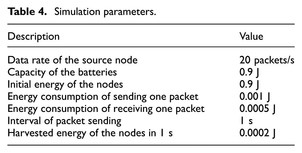
Scenario 5. Apply the DMF and EB-DMF routing algorithm in a regular network where $N = 4$ and $depth = 2$ . The data rate was fixed at $20 packets / s$ and the energy-harvesting rate of the nodes varied. The changes in load flow and network lifetime were observed.

Table 4.

Simulation parameters.

Description	Value
Data rate of the source node	20 packets/s
Capacity of the batteries	0.9 J
Initial energy of the nodes	0.9 J
Energy consumption of sending one packet	0.001 J
Energy consumption of receiving one packet	0.0005 J
Interval of packet sending	1 s
Harvested energy of the nodes in 1 s	0.0002 J

Simulation results

Table 5 shows the simulated load flow, and Table 6 shows the simulated network lifetime with different topology structures and a fixed node number $N = 200$ in a regular network. The load flow of FF, DMF, and EB-DMF increases with decreasing depth, and the network lifetime of DMF and EB-DMF is extended. A greater depth denotes an augmenting path from source node to destination node passing through more nodes. For EHWSN, the nodes not included in the augmenting path only harvest energy and do not consume energy during delivery of each packet. As a result, networks with a greater depth have smaller load flows and shorter network lifetimes. It is clear that the load flow of the network increases significantly with the use of the DMF and EB-DMF routing algorithm, and the EB-DMF routing algorithm prolongs the network lifetime compared to the DMF routing. The EB-DMF routing algorithm balances the flow distribution, so the energy consumption of the nodes is balanced and the network lifetime is extended. Table 7 shows the simulated load flow, and Table 8 shows the simulated network lifetime with increasing node number and fixed $depth = 5$ in a regular network. The fixed depth means the number of nodes through which the augmenting path passes does not change. The number of increasing nodes indicates the number of increasing same layer nodes, which means that the network has more augmenting paths and a larger load flow. Due to the increase in the augmenting path, more nodes are harvesting energy during every packet delivery interval, so the network lifetime is extended.

Table 5.

Load flow as a function of different topology structures with $N = 200$ .

Structure	FF	DMF	EB-DMF
2×100	1200	1200	1200
4×50	2200	2208	2424
5×40	2800	2952	3048
10×20	5800	5832	6240
20×10	11,800	12,600	13,152
40×5	13,152	26,568	29,664
50×4	29,664	34,104	40,536
100×2	59,800	93,912	129,576

FF: Ford–Fulkerson; DMF: dynamic maximum flow; EB-DMF: energy balanced dynamic maximum flow.

Table 6.

Network lifetime as a function of different topology structures with $N = 200$ .

Structure	DMF (s)	EB-DMF (s)
2×100	51	52
4×50	93	102
5×40	124	129
10×20	244	261
20×10	526	549
40×5	1108	1237
50×4	1422	1690
100×2	3914	5400

DMF: dynamic maximum flow; EB-DMF: energy balanced dynamic maximum flow.

Table 7.

Load flow as a function of the number of nodes with $depth = 5$ .

Number of nodes	FF	DMF	EB-DMF
20×5	11800	12648	13056
30×5	17800	19416	21096
40×5	23800	26568	29664
50×5	29800	35256	39600
60×5	35800	41904	52104
70×5	41800	53280	66720
80×5	47800	65448	82440

FF: Ford–Fulkerson; DMF: dynamic maximum flow; EB-DMF: energy balanced dynamic maximum flow.

Table 8.

Network lifetime as a function of the number of nodes with $depth = 5$ .

Number of nodes	DMF (s)	EB-DMF (s)
20×5	528	545
30×5	810	880
40×5	1108	1237
50×5	1470	1651
60×5	1747	2172
70×5	2221	2781
80×5	2728	3436

DMF: dynamic maximum flow; EB-DMF: energy balanced dynamic maximum flow.

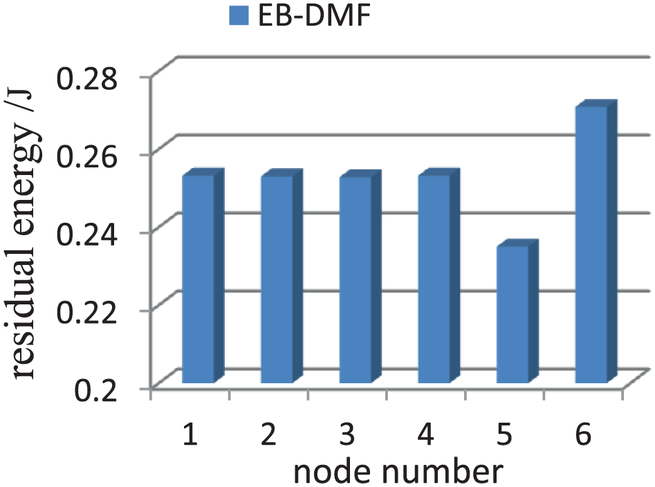
Figure 12 shows the residual energy distribution plotted against the node index for the regular network with $N = 200$ and $depth = 4$ when the first failure node appears (because of energy depletion) in the EB-DMF and DMF routing algorithms. The network life ends when DMF is used due to the unbalanced flow distribution, which results in nodes that pass through the augmenting path with larger flow consuming more energy than other nodes. The EB-DMF routing algorithm balances the energy consumption of nodes by changing the update time of edge capacities. The average residual energy of the nodes in EB-DMF is larger than in DMF, and EB-DMF has a more uniform residual energy distribution than the DMF routing algorithm. As a result, the lifetime of the EB-DMF network is longer than that of DMF. From Table 9, the network using the EB-DMF routing algorithm has more total energy than the network using the DMF routing algorithm. This is caused by the unbalanced energy consumption of nodes in DMF.

Figure 12.

The distribution of residual energy plotted as a function of the node index, for a regular network where $N = 200$ and $depth = 4$ , when the first failure node appears, for both EB-DMF and DMF routing algorithms.

Table 9.

Total energy comparison between EB-DMF and DMF when the first failure node appears, for the regular network where $N = 200$ and $depth = 4$ .

	EB-DMF	DMF
Total energy of the network (except virtual nodes) (J)	31.1960	8.0268

DMF: dynamic maximum flow; EB-DMF: energy balanced dynamic maximum flow.

The DMF algorithm sends packets along one augmenting path until there is no residual flow, then finds another augmenting path to transmit packets during the edge capacity updating period, which results in nodes not passing through the augmenting path continually harvesting energy and rapidly reaching their energy limit. The EB-DMF algorithm chooses the node with max residual energy as its next hop, which balances energy consumption among the nodes. The nodes do not reach their energy limit and harvest more energy. Thus, the network using the EB-DMF algorithm has a larger total energy. Taking Figure 2 as an example.

In DMF, from Table 2, it can be seen that the packets are delivered along $r_{1}^{1} {n_{s}, n_{1}, n_{4}, n_{D}}$ during the period from $t = 1$ to $t = 13$ , and nodes 1 and 4 continually consume energy. Theoretically, nodes 2, 3, 5, and 6 should harvest energy during this period. However, the energy of those nodes reaches the battery capacity, which limits them in storing harvested energy. In EB-DMF, the packets are delivered along ${r_{1}^{1}, r_{2}^{1}, r_{3}^{1}}$ in return. All the nodes quickly develop an energy gap and can harvest and store energy due to the balanced energy consumption among the nodes. To validate the performance of the proposed algorithm in realistic networks and to gain insight into which applications are better suited to the proposed routing algorithm, we can apply the algorithms to the BA and WS networks.

As shown in Table 10, the load flow clearly improved after using the DMF and EB-DMF algorithms. The network lifetime of the EB-DMF algorithm is significantly extended compared to the DMF algorithm, as shown in Table 11. In the two network models, the load flow has an increasing tendency while the total number of sensor nodes increases because more augmenting paths means more nodes are harvesting energy during each packet delivery interval.

Table 10.

Comparison of load flow of FF, DMF, and EB-DMF routing algorithms in WS and BA network models.

Number of nodes	WS			BA
	FF	DMF	EB-DMF	FF	DMF	EB-DMF
100	6551	6768	6960	3467	3576	4848
150	5974	6144	6288	3960	4296	4848
200	6551	6768	6960	7904	8688	9456
250	5948	6144	6288	9581	11,064	11,496
300	6550	6768	6960	14,987	16,632	17,736
350	7160	7416	7632	19,787	26,112	27,672
400	7752	8064	8232	24,521	36,048	40,392

FF: Ford–Fulkerson; DMF: dynamic maximum flow; EB-DMF: energy balanced dynamic maximum flow; WS: Watts–Strogatz; BA: Barabasi–Albert.

Table 11.

Network lifetime of FF, DMF, and EB-DMF routing algorithms in WS and BA network models.

Number of nodes	WS		BA
	DMF	EB-DMF	DMF	EB-DMF
100	284	292	150	203
150	258	263	180	203
200	284	292	363	395
250	258	264	462	480
300	284	292	695	741
350	311	320	1089	1154
400	338	344	1503	1684

FF: Ford–Fulkerson; DMF: dynamic maximum flow; EB-DMF: energy balanced dynamic maximum flow; WS: Watts–Strogatz; BA: Barabasi–Albert.

Meanwhile, the load flow of the WS model is larger than that of the BA model when using the same routing algorithms with the same number of sensor nodes, on the condition that the network is relatively small. In turn, the load flow of the WS model is smaller than that of the BA model when the network is large. Moreover, the load flow of the BA model increases more obviously than that of the WS model when the total number of nodes increases.

Figures 13 and 14 show the distribution of the residual energy of EB-DMF and DMF when the first failure node appears in the small-world and scale-free networks when $N = 200$ and the degree distribution is set to 4. By comparing Figures 13 and 14, it can be seen that the EB-DMF routing algorithm is more efficient in the BA network when the network consists of 200 nodes. EB-DMF has a more uniform residual energy distribution than the DMF routing algorithm in the BA network, while this cannot be seen in the WS network. Moreover, from Table 12, the total energy of EB-DMF is larger than that of DMF in both the BA WS networks. As a result, the EB-DMF routing algorithm has a longer network lifetime than DMF in both networks.

Figure 13.

The distribution of residual energy plotted as a function of the node index, for a small-world network where $N = 200$ and the degree distribution is set to 4, when the first failure node appears, for both EB-DMF and DMF routing algorithms.

Figure 14.

The distribution of residual energy plotted as a function of the node index, for a scale-free network where $N = 200$ and the degree distribution is set to 4, when the first failure node appears, for both EB-DMF and DMF routing algorithms.

Table 12.

Total energy comparison between EB-DMF and DMF when the first failure node appears, for a small-world network and scale-free network where $N = 200$ and the degree distribution is set to 4.

	WS		BA
	EB-DMF	DMF	EB-DMF	DMF
Total energy of the network (except the virtual nodes) (J)	153.1146	151.2056	142.9387	142.8742

DMF: dynamic maximum flow; EB-DMF: energy balanced dynamic maximum flow; WS: Watts–Strogatz; BA: Barabasi–Albert.

Although the EB-DMF algorithm can extend the load flow and prolong the network lifetime of both network models, it is more suitable for the BA model when the network is large and it is more suitable for the WS model when the network is small.

It is possible to draw a number of conclusions from these simulation scenarios. First, the DMF and EB-DMF routing algorithms, which dynamically update the capacity of the max flow algorithm, can extend the load flow of a network; the EB-DMF algorithm that balances the energy consumption among the nodes can actually prolong the lifetime of a network. Second, EB-DMF routing algorithm performs better in scale-free networks, with the same degree of distribution in a small-world network and a scale-free network when the network is large. In turn, the EB-DMF routing algorithm performs better in small-world networks when the network is small.

Figures 15 and 16, respectively, show the load flow and the network lifetime plotted as a function of the harvested energy of the nodes in 1 s for regular network where $N = 4$ and $depth = 2$ (as shown in Figure 2), when the first failure node appears, for both EB-DMF and DMF routing algorithms. When the data rate is fixed at 20 packets/s, with the energy-harvesting rate of the nodes increasing, the load flow and network lifetime extended. The energy-harvesting rate of the nodes increased, the nodes can harvest more energy between the packet sending intervals. There, the nodes can forward more packets. As a result, the load flow of the network increased. Moreover, the data rate remained unchanged, the increased energy-harvesting rate made the network tend to energy sustainability. The simulation results showed that the network was energy sustainable when the harvested energy of the nodes in 1 s reached 0.0104 J/s. In spite of the changing energy-harvesting rate of the nodes, the EB-DMF routing algorithm had advantage over DMF routing algorithm in extending the load flow and the network lifetime.

Figure 15.

The load flow plotted as a function of the harvested energy of the nodes in 1 s, for regular network where $N = 4$ and $depth = 2$ (as shown in Figure 2), when the first failure node appears, for both EB-DMF and DMF routing algorithms.

Figure 16.

The network lifetime plotted as a function of the harvested energy of the nodes in 1 s, for regular network where $N = 4$ and $depth = 2$ (as shown in Figure 2), when the first failure node appears, for both EB-DMF and DMF routing algorithms.

Conclusion and future works

We proposed an EB-DMF routing algorithm for EHWSN based on the max flow algorithm and investigated the flow load and the network lifetime assuming that all nodes had the same initial energy and energy-harvesting rate. The proposed routing algorithm considers realistic network structures and the dynamic energy variation of EHWSN.

Our proposed algorithm improves upon the FF algorithm in both the extension of the load flow and the network lifetime. First, our algorithm dynamically updates the capacity according the residual energy of the nodes considering the energy harvested by the nodes. Second, the flow distribution of FF is not balanced, leading to unbalanced energy consumption in the nodes. The update time is changed to achieve balanced energy consumption among the nodes and prolong the network lifetime.

Because of these two improvements, EB-DMF extends the load flow and the network lifetime. Our algorithms were applied to a regular network, a BA network, and a WS network, and the comparison provided information on application scenarios.

In future work, we will improve and extend the EB-DMF algorithms, taking other factors into account. First, we will consider different energy-harvesting rates in nodes, and second, we will consider a sleep–awake mechanism in nodes to prolong the network lifetime.

Footnotes

Handling Editor: Chang Wu Yu

Declaration of conflicting interests

The author(s) declared no potential conflicts of interest with respect to the research, authorship, and/or publication of this article.

Funding

The author(s) disclosed receipt of the following financial support for the research, authorship, and/or publication of this article: This work was supported in part by the National Natural Science and Foundation of China under Grants 61702369 and Tianjin Municipal Science and Technology Commission under Grant 15JCYBJC52400.

References

Shaikh

Zeadally

. Energy harvesting in wireless sensor networks: a comprehensive review. Renew Sust Energ Rev 2016; 55: 1041–1054.

Wang

Niyato

et al . Wireless networks with RF energy harvesting: a contemporary survey. IEEE Commun Surv Tut 2015; 17(2): 757–789.

Smith

Faucheaux

Jain

. Plasmon resonances for solar energy harvesting: a mechanistic outlook. Nano Today 2015; 10(1): 67–80.

Yang

. Thermal energy harvesting for WSNs. In: 2010 IEEE international conference on systems man and cybernetics (SMC), Istanbul, 10–13 October 2010, pp.3045–3052. New York: IEEE.

Patil

Reddy

. Design and development of low frequency vibration energy harvester for wireless sensor networks. Procedia Engineer 2016; 144: 607–612.

Bogliolo

Lattanzi

Acquaviva

. Energetic sustainability of environmentally powered wireless sensor networks. In: Proceedings of the 3rd ACM international workshop on performance evaluation of wireless ad hoc, sensor and ubiquitous networks, Malaga, 06–06 October 2006, pp.149–152. New York: ACM.

Lattanzi

Regini

Acquaviva

et al . Energetic sustainability of routing algorithms for energy-harvesting wireless sensor networks. Comput Commun 2007; 30(14): 2976–2986.

Seraghiti

Bogliolo

. Self-adapating maxflow routing for autonomous wireless sensor networks. In: International conference on sensor technologies and applications (Sensorcomm ’08), Cap Esterel, 25–31 August 2008, pp.360–365. New York: IEEE.

Bogliolo

Delpriori

Lattanzi

et al . Self-adapting maximum flow routing for autonomous wireless sensor networks. Cluster Comput 2011; 14(1): 1–14.

10.

Liu

. Routing protocol based on genetic algorithm for energy harvesting-wireless sensor networks. IET Wirel Sens Syst 2013; 3(2): 112–118.

11.

Watts

Strogatz

. Collective dynamics of “small-world” networks. Nature 1998; 393(6684): 440–442.

12.

Barabási

Albert

. Emergence of scaling in random networks. Science 1999; 286(5439): 509–512.

13.

Meng

Zhang

Dong

et al . Adaptive energy-harvesting aware clustering routing protocol for wireless sensor networks. In: 2012 7th international ICST conference on communications and networking in China (CHINACOM), Kun Ming, China, 8–10 August 2012, pp.742–747. New York: IEEE.

14.

Voigt

Ritter

Schiller

. Solar-aware routing in wireless sensor networks. In: IFIP international conference on personal wireless communications. Berlin, Heidelberg: Springer, 2003, pp.847–852.

15.

Voigt

Dunkels

Alonso

et al . Solar-aware clustering in wireless sensor networks. In: Proceedings ISCC 2004. Ninth international symposium on computers and communications, Alexandria, 28 June–1 July 2004, pp.238–243. New York: IEEE.

16.

Islam

. A-sLEACH: an advanced solar aware leach protocol for energy efficient routing in wireless sensor networks. ICN 2007; 7: 4.

17.

Tan

. Adaptive opportunistic routing protocol for energy harvesting wireless sensor networks. In: 2012 IEEE international conference on communications (ICC), Ottawa, ON, Canada, 10–15 June 2012, pp.318–322. New York: IEEE.

18.

Girvan

Newman

MEJ

. Community structure in social and biological networks. Proceedings of the National Academy of Sciences of the United States of America 2002; 99(12): 7821–7826.

19.

Reka

Jeong

Barabasi

. Diameter of the world-wide web. Nature 1999; 401(6749): 130–131.

20.

Huberman

Adamic

. Growth dynamics of the world-wide web. J Reprod Fertil 1993; 9: 55–60.

21.

Ruela

Cabral

Aquino

ALL

et al . Evolutionary design of wireless sensor networks based on complex networks. In: 2009 5th international conference on intelligent sensors, sensor networks and information processing (ISSNIP), Melbourne, VIC, Australia, 2009, pp.237–242. New York: IEEE.

22.

Guan

. Energy-aware routing in wireless sensor networks using local betweenness centrality. Int J Distrib Sens N 2013; 9(5): 213–235.

23.

Zhang

Liang

Jiang

et al . Improved efficient static weighted routing strategy on two-layer complex networks. Int J Mod Phys C 2015; 26(1): 1550001.

24.

Han

Guo

et al . Improved efficient routing strategy on two-layer complex networks. Int J Mod Phys C 2016; 27(4): 1650044.

25.

Lin

Chen

Gao

et al . Advanced algorithms for local routing strategy on complex networks. PLoS ONE 2016; 11(7): e0156756.

26.

Yang

Fan

Tang

WKS

. Routing design for transmission capacity maximization in complex networks. In: 2015 IEEE international symposium on circuits and systems (ISCAS), Lisbon, 24–27 May 2015, pp.1482–1485. New York: IEEE.

27.

Murali

Ordóñez

Dessouky

. Modeling strategies for effectively routing freight trains through complex networks. Transport Res C: Emer 2016; 70: 197–213.

28.

Anastasi

Conti

Di Francesco

et al . Energy conservation in wireless sensor networks: a survey. Ad Hoc Netw 2009; 7(3): 537–568.

29.

Peng

Awad

et al . Energy-efficient and fault-tolerant evolution models for large-scale wireless sensor networks: a complex networks-based approach. In: 2015 IEEE global communications conference (GLOBECOM), San Diego, CA, 6–10 December 2015, pp.1–6. New York: IEEE.

Dynamic energy balanced max flow routing in energy-harvesting sensor networks

Abstract

Keywords

Introduction

Related works

Routing in EHWSN

Routing in complex networks

Network environment and problem formulation

Network environment

Problem formulation

Routing algorithm

FF algorithm

DMF routing algorithm

Energy balanced dynamic max flow routing algorithm

Simulation

Simulation model

BA model

WS model

Simulation scenarios

Simulation results

Conclusion and future works

Footnotes

Declaration of conflicting interests

Funding

References