Joint routing and scheduling for data collection with compressive sensing to achieve order-optimal latency

Abstract

We consider a joint routing and scheduling scheme for data collection in wireless sensor networks leveraging compressive sensing under the protocol interference model. We propose the construction of a connected dominating set as a network backbone for efficient routing. A hybrid compressive sensing technique, which combines conventional and compressive data gathering schemes, is used to aggregate data over the backbone. Pipelined scheduling is developed for fast aggregation of compressed data over the backbone. We set the communication range of sensor nodes to an appropriate value to control the size of the backbone and demonstrate that the proposed scheme can achieve order-optimal latency for data gathering. We extend the proposed scheme to the physical interference model and show that comparable latency is achievable under physical interference model. In addition, the proposed scheme is shown to be energy-efficient, in that it can achieve order-optimal energy consumption given that the sensor data sparsity is of constant order. Simulation results show the effectiveness of the proposed scheme in terms of latency and energy consumption.

Introduction

Wireless sensor networks (WSNs) consist of low-cost and energy-constrained sensors that acquire and transmit environmental and contextual information to a data sink. WSNs are a key element in the emerging Internet of Things technology. ¹ Timely transmission of sensed data to the sink is important, particularly for applications such as emergency/catastrophe monitoring systems or mission-critical networks, which require low or strictly bounded latency for data collection. In this article, we consider a joint routing and scheduling scheme for data collection with compressive sensing (CS), which achieves order-optimal latency. The CS technique was originally proposed in the signal-processing literature; however, it has recently been applied to efficient data collection. The idea behind CS is to reliably recover a high-dimensional signal, that is, the original data vector, from a significantly smaller number of measurements. ² Surprisingly, exact recovery is possible with linear and non-adaptive measurements, which enables efficient sensing for data acquisition.^2–5

Efficient collection of sparse data under the CS framework has attracted considerable attention. For example, Luo et al. ⁶ proposed compressive data gathering (CDG) to collect data in WSNs using CS. In CDG, the sink collects linear combinations of sensed data rather than collecting all data samples individually. Once a sufficient number of linear combinations is collected, the sink can recover the original sparse data vector by solving an l₁-based convex optimization problem. ² The main advantage of CDG is that it reduces sensor-node energy consumption and evenly distributes loads across the network. However, Luo et al. ⁷ showed that applying CS naively, for example, CDG, may not improve performance because in CDG, nodes that are distant from the sink, for example, leaf nodes, may transmit more data (for $m$ times) than those in the conventional data gathering scheme (for one time for leaf nodes). Luo et al. proposed a hybrid CS scheme that encodes data only at overloaded nodes, for example, nodes close to the sink, unlike CDG, in which encoding is performed at each sensor. They demonstrated that the hybrid CS scheme can further improve throughput. Under the CDG framework, Ebrahimi and Assi ⁸ considered not only energy consumption but also latency of data gathering. They formulated a joint optimization problem to collect data at the sink with both minimal latency and fewer transmissions. In addition, they proved that the problem was non-deterministic polynomial-time (NP)-hard. They also proposed a two-approximation method, which decomposes the problem into forwarding tree construction and link-scheduling subproblems. However, their scheme used the original CDG without modification. In contrast, the proposed scheme utilizes the hybrid CS scheme and considers both latency and energy aspects of data collection. Zheng et al. ⁹ studied the capacity and delay of CS-based techniques for data gathering in WSNs under the CDG framework. They also considered the protocol interference model (PrIM).^9,10 For a single sink case, they proposed a data gathering scheme that can achieve $\Theta (\mathrm{nW}/k\log n)$ capacity and $\Theta (k\sqrt{n\log n})$ latency, where $n$ is the number of sensors in the network, $W$ is the capacity of each link, and $k$ is the sparsity of the data vector. However, a limitation of capacity-achieving schemes, such as the study of Zheng et al., ⁹ is that the schemes are typically built for regular-shaped networks, such as square networks. These schemes rely on a certain geometric structure of the network and node locations. However, practical WSNs may be deployed in an area with a highly irregular shape and node density. In contrast, we employ a graph-theoretic approach for joint routing and scheduling based on techniques proposed by Wan et al. ¹¹ This enables implementation of the proposed routing and scheduling scheme for networks of arbitrary shapes and topologies.

Recently, the energy efficiency of CS-based data gathering has been studied for WSNs. Karakus et al. ¹² compared the energy performance of CS-based schemes to conventional schemes under an energy dissipation model that considers the energy consumption of data acquisition, processing, and communication. Their measurement study using MICA motes demonstrated that network lifetime can be increased by applying CS to WSN data gathering. Under the CDG framework, Zhao et al. ¹³ observed that determining the sparsity of raw data in WSNs may not be straightforward due to the randomness of sensor distribution. They proposed an energy-efficient treelet-based clustered compressive data aggregation (T-CCDA) scheme that jointly considers the sparsification basis and data aggregation routing. In T-CCDA, a treelet transform is adopted to determine the sparsity from the raw data, and a clustered routing algorithm is proposed to further facilitate energy-saving. Liu et al. ¹⁴ proposed a nonuniform random projection-based estimation algorithm for compressive data collection using a power-law decaying data model under the CDG framework. Their scheme required fewer compressed measurements and allowed a simple routing strategy without excessive computation and overhead. They proved that their algorithm could achieve the optimal estimation error bound. Zhao et al. ¹³ and Liu et al. ¹⁴ both used CDG without modification, that is, each node in the data collection path must compress data. However, we construct a backbone for routing and aggregate the data over the backbone using the hybrid CS technique. This reduces the total number of transmissions in the network, which leads to further energy-savings because the backbone tends to be relatively small. Xu et al. ¹⁵ observed that hybrid CS utilizes only a small fraction of sensors due to inefficient network configurations. They proposed hierarchical data aggregation using compressive sensing (HDACS) based on an energy model that captures both processor and radio energy consumption. The idea behind HDACS is to optimize data transmissions by setting multiple compression thresholds adaptively based on cluster sizes at different levels of the data aggregation tree. However, latency is not considered in their scheme.

In this article, we propose a CS-based data collection scheme for low latency and energy consumption. The proposed scheme exploits the graph-theoretic structure of the underlying network, which we refer to as the connected dominating set (CDS). We construct a network backbone for efficient routing using the CDS and develop a joint routing and scheduling scheme. We leverage the hybrid CS technique such that raw data from non-backbone nodes are aggregated to the backbone. Then, linearly combined data are routed and scheduled over the backbone in a pipelined manner. Since the proposed scheme is based on a network graph, it differs from previous schemes based on particular network geometry, for example, square networks, ⁹ as follows. (1) The proposed scheme can be implemented on networks of arbitrary shapes and topologies; thus, it is more general than schemes designed for square networks. (2) The proposed scheme leverages a network graph induced from the spatial node distribution; thus, it can construct a smaller backbone compared to those based on square networks. Simulation results show that the proposed approach leads to less latency and energy consumption.

To demonstrate the efficiency of the proposed scheme theoretically, we analyze its performance on a random planar network. The scheme achieves latency given by $\Theta (k\log n+\sqrt[3]{n})$ with high probability, which improves the result $\Theta (k\sqrt{n\log n})$ obtained by Zheng et al. ⁹ Moreover, this latency is order-optimal (given by $\Theta (\sqrt[3]{n})$ ) provided that $k=O(\sqrt[3]{n}/\log n)$ , which is commonly assumed for sparsity $k$ in the CS literature. We extend the proposed scheme to the physical interference model (PhIM), in which all receivers must satisfy a predetermined signal-to-interference-plus-noise ratio (SINR) requirement. We demonstrate that the proposed scheme is also energy-efficient, by showing that the total number of transmissions in the network is small. It is proved that our scheme consumes at most $O(k+1)$ times the minimum energy, implying that it is order-optimal if $k=O(1)$ . We perform a simulation to evaluate the energy performance of the proposed scheme and show that it outperforms the existing methods. In particular, the proposed scheme shows superior performance relative to energy consumption even when $k$ grows faster than $O(1)$ .

The contributions of this article can be summarized as follows:

• A graph-based algorithm is developed under PrIM and can be applied to networks of arbitrary shapes and topologies, unlike many conventional schemes that assume a specific network geometry, for example, square networks. ⁹

• The proposed scheme achieves order-optimal latency for data collection under PrIM.

• We extend our scheme to PhIM ¹⁰ and show that comparable latency is achievable.

• The proposed scheme is shown to achieve order-optimal energy consumption if data sparsity is $O(1)$ . Simulation results show that the proposed scheme has good energy performance even when data sparsity grows faster than $O(1)$ .

The remainder of this article is organized as follows. We introduce the system model in section “System model.” In section “Proposed scheme,” we describe the proposed data collection scheme. Analysis of the proposed scheme for a random square network is presented in section “Latency analysis.” Section “PhIM” extends our scheme to a PhIM. Energy consumption is discussed in section “Energy consumption.” Simulation results are provided in section “Simulations,” and conclusions and suggestions for future work are presented in section “Conclusion and future work.”

System model

Here, we briefly introduce the CS technique, where the following linear model is considered

$$\mathbf{y}=\mathbf{Ax}$$

(1)

where $\mathbf{y}\in {\mathbb{R}}^m$ is the measurement vector, $\mathbf{x}\in {\mathbb{R}}^n$ is the original data vector, and $\mathbf{A}\in {\mathbb{R}}^{m\times n}$ is referred to as the sensing matrix. A vector $\mathbf{x}$ is considered k-sparse in a basis $\mathbf{\Psi }$ if $\mathbf{x}=\mathbf{\Psi }\mathbf{c}$ , and the number of nonzero entries in $\mathbf{c}$ does not exceed $k$ . In CS, the sensing matrix $\mathbf{A}$ is typically a random matrix. Note that a Gaussian random matrix is widely used, that is, each entry of $\mathbf{A}$ is drawn i.i.d. from the Gaussian distribution $N(0,1/m)$ . It is known that if $m=O(k\log (n))$ and $k<<n$ , a k-sparse vector $\mathbf{x}$ can be recovered with high probability via linear programming.^2,16 In this article, we assume that the original data vector can be reliably recovered if a sufficient number of measurements are gathered at the sink. We focus on the efficient collection of a given number of measurements from the sensors.

Here, we consider a network with $n$ sensors $v_1,v_2,\dots ,v_n$ deployed in an area where $v_1$ is the sink node. Sensor $v_i$ acquires a reading denoted by $x_i$ . The collection of sensor readings, that is, $\mathbf{x}=[x_1,\dots ,x_n]$ , is referred to as the data vector. We assume that all nodes in the network share a common wireless channel. We denote the Euclidian distance between node $v_i$ and $v_j$ as $|v_i-v_j|$ . We consider a time-slotted system wherein time slots are of equal duration and assume that a node can transmit a unit-size packet during each time slot. In this article, PrIM is considered as follows. We assume a common range $r$ for node transmissions. Node $v_i$ can successfully transmit data to $v_j$ if (1) $|v_i-v_j|\le r$ and (2) $|v_k-v_j|\ge (1+\delta )r$ for concurrent transmitters $v_k$ , where $\delta >0$ is a constant. In PrIM, any two transmitters that are at least $\rho r$ distant from each other, where $\rho =(2+\delta )$ , can transmit data simultaneously. We construct a communication graph $G=(V,E)$ induced by PrIM where $V:=\{v_1,v_2,\dots ,v_n\}$ , and an edge $(v_i,v_j)\in E$ exists if $|v_i-v_j|\le r$ .

Next, we briefly describe how to apply CS to data collection. In CS, the linear model $\mathbf{y}=\mathbf{Ax}$ is considered, where $\mathbf{y}\in {\mathbb{R}}^m$ is the measurement vector, $\mathbf{x}\in {\mathbb{R}}^n$ is the original data vector, and $\mathbf{A}\in {\mathbb{R}}^{m\times n}$ is the sensing matrix. A signal $\mathbf{x}$ is said to be k-sparse in basis $\mathbf{\Psi }$ if $\mathbf{x}=\mathbf{\Psi }\mathbf{c}$ , and the number of nonzero entries in $\mathbf{c}$ does not exceed $k$ . Assume $\mathbf{A}$ is a Gaussian random matrix, that is, each entry of $\mathbf{A}$ is drawn i.i.d. according to the Gaussian distribution $N(0,1/m)$ . If $m=O(k\log (n))$ and $k<<n$ , $\mathbf{x}$ can be recovered from linear combinations $y_j=\sum _{i=1}^n{a}_{\mathrm{ji}}{x}_i,$ $j=1,\dots ,m,$ where $a_{\mathrm{ij}}$ denotes the $(i,j)\mathrm{th}$ element of $\mathbf{A}$ with high probability via linear programming. ²

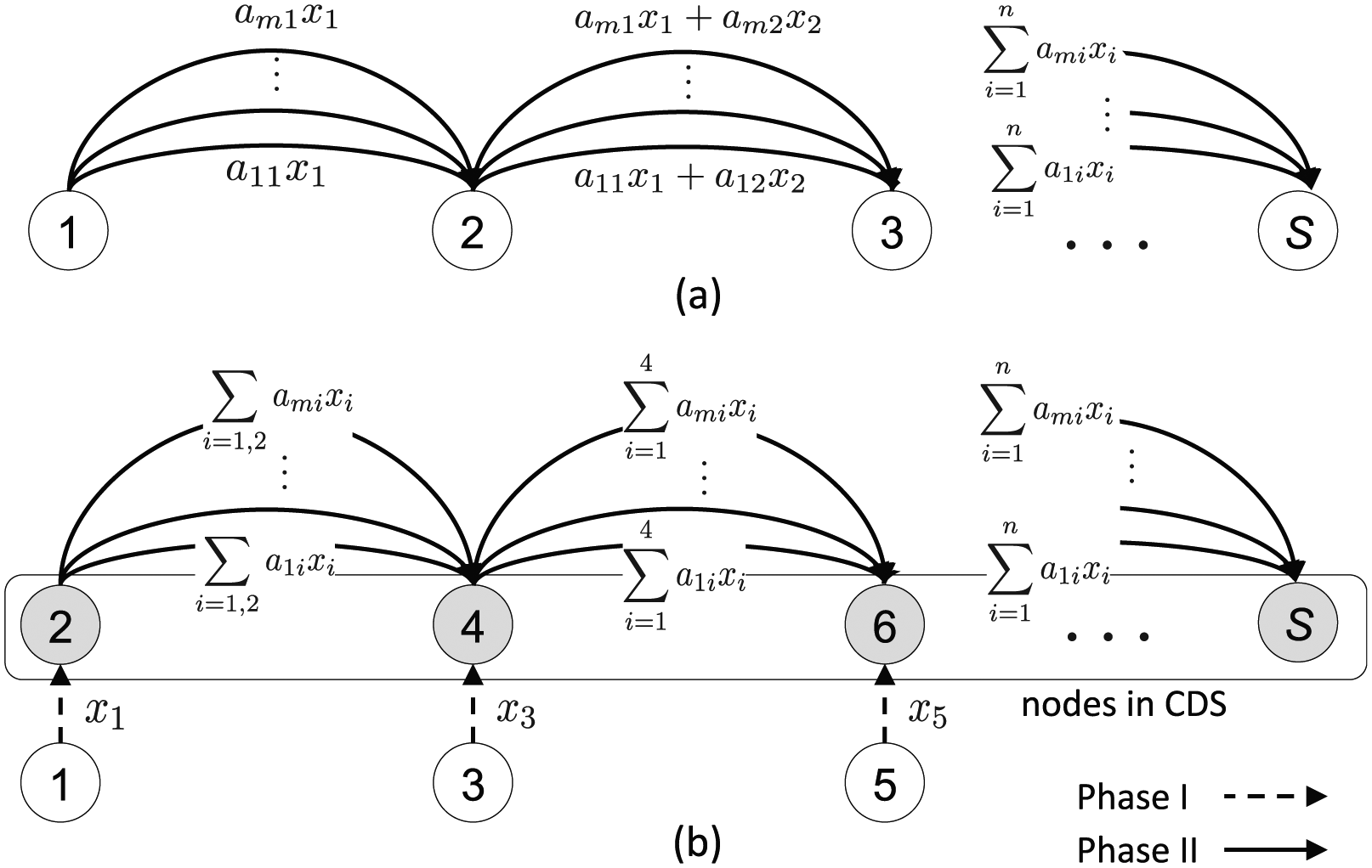
Figure 1(a) shows CDG, in which each node combines its data linearly with the data received from the node at the previous hop. The number of transmissions at any link is $m$ ; thus, CDG only requires a few transmissions per link and balances the load across the network.

Figure 1.

Comparison of: (a) CDG and (b) proposed scheme for linear networks. Shaded nodes belong to CDS.

Proposed scheme

In the proposed scheme, we first construct a backbone that consists of nodes with a large transport gain, that is, the backbone enables efficient routing to the sink in a relatively small number of hops. Next, we schedule data collection in two phases. In Phase I, non-backbone nodes transmit raw data to the backbone. In Phase II, backbone nodes transmit linearly combined data toward the sink in a pipelined manner. Thus, the pipelined data aggregation takes place only among the backbone nodes, which can substantially reduce latency. An outline of the proposed scheme is shown in Figure 1.

Our scheduling method is inspired by hybrid CS proposed by Luo et al.; ⁷ however, the key differences are (1) backbone construction leveraging CDS, (2) pipelined scheduling over the backbone, and (3) the backbone is constructed based on a graph-theoretic framework; thus, the algorithm can be applied to networks of arbitrary shape and topology, whereas Luo et al. ⁷ outlined a scheme for square networks.

Routing

Here, we consider routing in the proposed scheme. First, we present some definitions.

Definition 1

A subset $U\subseteq V$ is a dominating set of $G$ if each node in $V-U$ is adjacent to some node in $U$ . $U$ is a CDS if the subgraph induced by $U$ is connected.

Definition 2

A subset $U\subseteq V$ is an independent set (IS) of $G$ if no two nodes in $U$ are adjacent.

Definition 3

An IS $U$ is a maximal independent set (MIS) of $G$ if $U\cup \{v\}$ is not an IS for any $v\in V-U$ .

Definition 4

The radius of $G$ , denoted by $R$ , is given by $R=\underset{v_i\in V}{max}P(v_i,v_1)$ , where $P(v_i,v_1)$ denotes the distance of the shortest path between $v_i$ and sink node $v_1$ .

We adopt a widely used method proposed by Wan et al. ¹¹ to construct the CDS as follows. Given $G$ , we first find an MIS $I$ in which nodes are referred to as dominators. Then, we divide $I$ into the following levels. Let $H$ be the graph induced by $I$ where an edge between two dominators exists if and only if they share a common neighbor in $G$ . The radius of $H$ is denoted $R$ . Level $I_j\subseteq I(0\le j\le R)$ consists of dominators of depth $j$ in $H$ . Next, we connect two adjacent levels $I_j$ and $I_{j+1}$ as proposed by Wan et al. ¹¹ Suppose $W_j$ is the set of nodes that connect $I_{j-1}$ and $I_j$ . The nodes in $W:={\cup }_j{W}_j$ are called connectors. CDS is given by $I\cup W$ . Based on the distance to the sink, the increasing order of levels in CDS is given by $I_0,W_1,I_1,W_2,\dots ,W_R,I_R$ . Finally, the set of non-CDS nodes is denoted by $D:=V-I\cup W$ . We refer to non-CDS nodes as the dominatees. Figure 2 shows an example of the routing scheme.

Figure 2.

Proposed routing scheme.

The routing procedure is completed by designating the next-hop nodes for CDS and non-CDS nodes as follows:

• CDS nodes. Each node in CDS randomly selects a neighbor that belongs to the lower level as its receiving node. Specifically, a node in $I_j$ (resp. $W_j$ ) selects a neighbor in $W_j$ (resp. $I_{j-1}$ ) as its receiving node.

• Non-CDS nodes. Dominatee $v$ selects the closest dominator as its receiving node, denoted by $\mathrm{Re}(v)$ .

Scheduling

The scheduling procedure is divided into two phases (Algorithm 1).

Algorithm 1 Data Collection Scheduling

1: Input $G=(V,E)$ , $I,W,D,\rho ,r$ 2: Phase I: schedule transmissions between $D$ and $I$ .3: Construct a graph $G_D=(D,E_D)$ where an edge $(v_i,v_j)\in E_D$ exists if $|v_i-v_j|\le \rho r$ .4: Color nodes in $G_D$ such that any two adjacent nodes have different colors. Let $\tilde{c}$ be the total number of colors and $c(v)\in \{1,2,\dots ,\tilde{c}\}$ be the color of dominatee $v\in D$ .5: for $i=1$ $\tilde{c}$ do6:   Each dominatee $v$ with $c(v)=i$ transmits its raw data to $\mathrm{Re}(v)$ at the ith time slot.7: end for8: Phase II: schedule transmissions among the nodes in CDS.9: $X(I_j^i)$ :=(starting time of level Ij’s transmission during the ith round).10: $X(W_j^i)$ :=(starting time of level W j ’s transmission during the ith round).11: $X(I_R^1)=\tilde{c}+1$ /* Phase II starts at time slot $\tilde{c}+1$ */12: for $i=1$ $m$ do13:  for $j=R$ to $2$ do14:   $X(W_j^i)=X(I_j^i)+\lceil 4{\beta }_{\rho +1}\rceil$ .15:   $X(I_{j-1}^i)=X(W_j^i)+\lceil 11{\beta }_{\rho +1}\rceil$ .16:  end for17:   $X(W_1^i)=X(I_1^i)+\lceil 11{\beta }_{\rho +1}\rceil$ .18:   $X(I_R^{i+1})=X(I_{R-\lceil \rho \rceil }^i)$ .19: end for

In Phase I, we schedule the transmissions between dominatees and dominators. First, we construct the graph $G_D$ (Algorithm 1, line 3) and then color each node in $D$ such that no two adjacent nodes are the same color. Note that the Euclidian distance between $v_i\in D$ and $v_j\in D$ is greater than $\rho r$ if $(v_i,v_j)\notin E_D$ . Thus, $v_i$ and $v_j$ can transmit data concurrently. Each dominatee transmits the raw data to its receiving node. Thus, one transmission is sufficient for each dominatee to complete the data collection.

In Phase II, we adopt the CDG scheme to collect $m$ linear combinations of raw data. Specifically, the sink collects measurement $y_i,$ $i=1,2,\dots ,m,$ during the ith round. Each node in CDS transmits the linear combination of its data and those from its receiving nodes during each round. Note that a dominator may have the raw data of its corresponding dominatees, which are collected in Phase I. During each round, we schedule the transmissions of CDS nodes using sequential aggregation scheduling (SAS) ¹¹ for $\rho >1$ . SAS assigns $\lceil 4{\beta }_{\rho +1}\rceil$ time slots to $I_j$ and $\lceil 11{\beta }_{\rho +1}\rceil$ time slots to $W_j$ , where ${\beta }_{\rho +1}=(\pi /\sqrt{3})(\rho +1{)}^2+((\pi /2)+1)(\rho +1)+1$ . We also pipeline the transmissions between adjacent rounds based on levels. For example, $I_R$ can transmit at the $(i+1)\mathrm{th}$ round concurrently with $I_{R-\lceil \rho \rceil }$ at the ith round because the distance between the nodes in $I_R$ and $I_{R-\lceil \rho \rceil }$ is at least $\rho r$ .

Latency analysis

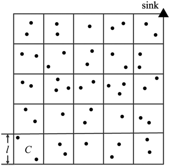
In this section, we analyze the latency performance of the proposed scheme. Although our scheme can be applied to networks of arbitrary shape and topology, it is difficult to analyze performance on arbitrary networks. Instead, for performance analysis, we consider a random planar network. Suppose $n$ sensors are deployed uniformly at random over a unit square where the sink is located at the top right corner (Figure 3). We demonstrate that the proposed scheme achieves order-optimal latency under this model. Throughout this section, we assume that $r\ge \Theta (\sqrt{\log n/n})$ , which ensures network connectivity. ¹⁷

Figure 3.

Partitions of the unit square network.

Lemma 1

For a large $n$ , the latency of any scheme under PrIM is at least $\Theta (\sqrt[3]{n})$ with high probability.

Proof 1

We divide the network into square cells of size $l\times l$ , where $l=\rho r/\sqrt{2}$ . Let $C$ be the cell located at the bottom left corner, that is, cell $C$ is farthest from the sink. Clearly, the overall latency of data collection is bounded below the worst latency experienced by a node in $C$ .

Let $Z$ be the number of nodes in $C$ . Here, $Z~B(n,l^2)$ , where $B(·,·)$ denotes binomial distribution. From Chebyshev’s inequality, for some $a\in (0,1/2)$ , we have

$$\begin{array}{cc}\multicolumn{1}{c}{\mathbb{P}(|Z-n{l}^2|\ge \sqrt{n}l(\log n{)}^a)}& \le \frac{n{l}^2(1-l^2)}{{\left\{\sqrt{n}l{(\log n)}^a\right\}}^2}\hfill \\ \multicolumn{1}{c}{}& \le \frac{1}{{(\log n)}^{2a}}\hfill \end{array}$$

(2)

From equation (2), for a large $n$ , the number of nodes in $C$ is $\Theta (n{l}^2)$ with high probability, which can be expressed as

$$\frac{n{l}^2}{\sqrt{n}l{(\log n)}^a}=\frac{\rho }{\sqrt{2}}\frac{\sqrt{n}r}{{(\log n)}^a}\ge \Theta \{(\log n{)}^{\frac{1}{2}-a}\}$$

(3)

where

$$l=\frac{\rho r}{\sqrt{2}}\ge \Theta \left(\sqrt{\frac{\log n}{n}}\right)$$

Thus, equation (3) implies that the variation in $Z$ centered at $n{l}^2$ in equation (2), which is given by $\sqrt{n}l(\log n{)}^a$ , is $o(n{l}^2)$ ; thus, $Z$ is $\Theta (n{l}^2)$ with high probability. Moreover, any two nodes in $C$ cannot transmit data simultaneously because their distance is less than $\rho r$ . Thus, it takes at least $\Theta (n{l}^2)=\Theta (n{r}^2)$ time slots to complete the transmissions in $C$ because all nodes in $C$ must transmit data at least once.

Now consider node $v$ , which is the last node to transmit in $C$ . Here, it must have waited for $\Theta (n{r}^2)$ time slots. In addition, the packet generated by $v$ must be relayed to the sink. However, for any packet generated within $C$ , it takes at least $\sqrt{2}(1-l)/r=\Theta (r^{-1})$ time slots to reach the sink. Thus, the total latency experienced by $v$ is at least $\Theta (n{r}^2+r^{-1})$ . The lemma is proved by “minimizing” $n{r}^2+r^{-1}$ with respect to $r$ or by letting $r=\Theta (n^{-1/3})$ , which yields latency of $\Theta (\sqrt[3]{n})$ .

Lemma 2

Suppose $r=\Theta (n^{-1/3})$ . For a large $n$ , the maximum degree $\Delta$ of nodes in $G_D$ is at most $\Theta (\sqrt[3]{n})$ with high probability.

Proof 2

Consider a dominatee $v\in D$ . The number of nodes in $B_{\rho r}(v)$ where $B_{\rho r}(v)$ is the disk rooted at $v$ and with radius $\rho r$ is denoted $N$ . Here, $N~B(n,\pi {\rho }^2{r}^2)$ . From Chebyshev’s inequality, for some $a\in (1/2,1)$

$$\begin{array}{cc}\multicolumn{1}{c}{\mathbb{P}(|N-\pi {\rho }^{2}n{r}^2|}& \ge {(n{r}^2)}^a)\le \frac{\pi n{\rho }^2{r}^2(1-\pi {\rho }^2{r}^2)}{{(n{r}^2)}^{2a}}\hfill \\ \multicolumn{1}{c}{}& \le \frac{\pi {\rho }^2}{{(n{r}^2)}^{2a-1}}\hfill \\ \multicolumn{1}{c}{}& =\Theta (n^{-\frac{2a-1}{3}})\hfill \end{array}$$

(4)

where equation (4) follows from the assumption that $r=\Theta (n^{-1/3})$ . This implies that for a large $n$ , the maximum degree of nodes in $G_D$ is at most $\Theta (n{r}^2)=\Theta (\sqrt[3]{n})$ with high probability.

Now, we are ready to prove our main theorem.

Theorem 1

Let $r=\Theta (n^{-1/3})$ . For a large $n$ , our scheme achieves latency $L=\Theta (k\log (n)+\sqrt[3]{n})$ with high probability. Thus, if $k=O(\sqrt[3]{n}/\log n)$ , $L$ is given by $\Theta (\sqrt[3]{n})$ , which is order-optimal.

Proof 3

Let us first consider the latency of Phase I. Brooks ¹⁸ showed that $\Delta +1$ colors are sufficient to color nodes in $D$ , where $\Delta$ is the maximum degree of nodes in $D$ , such that no two adjacent nodes receive the same color. Thus, from Lemma 2, the latency of Phase I is at most $\Theta (\sqrt[3]{n})$ time slots.

Next, we compute the latency of Phase II. Consider two dominators $v_i\in I_j$ and $v_j\in I_{j+1}$ . We observe that $|v_i-v_j|\in (r,2r]$ holds, which implies that the radius of $H$ is given by $R=\Theta (r^{-1})$ . In Phase II, the latency of each round is $\Theta (R+\Delta )=\Theta (r^{-1}+\Delta )$ . ¹¹ We pipeline the transmissions between adjacent rounds for $m$ rounds; thus, the latency of Phase II is $\Theta (m+r^{-1}+\Delta )=\Theta (k\log (n)+\sqrt[3]{n})$ from Lemma 2. Therefore, the overall latency $L$ is given by

$$\Theta (k\log (n)+\sqrt[3]{n})$$

which reduces to $\Theta (\sqrt[3]{n})$ if $k=O(\sqrt[3]{n}/\log n)$ . This completes the proof.

Finally, note that the optimal transmission radius $r=\Theta (n^{-1/3})$ is sufficient for network connectivity because it exceeds the critical transmission range, ¹⁷ that is, $r\ge \Theta (\sqrt{\log n/n})$ .

PhIM

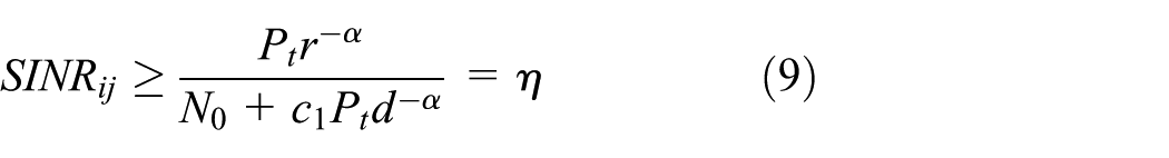
We extend the proposed scheme to PhIM. We assume that each node transmits data at a common transmit power denoted by $P_t$ . Under PhIM, receiver $v_j$ can successfully receive data from a transmitter $v_i$ if and only if the SINR in $v_j$ satisfies

$$\mathrm{SIN}{R}_{\mathrm{ij}}=\frac{P_t|v_i-v_j{|}^{-\alpha }}{N_0+\sum _{v_k\in S(v_i)}{P}_t|v_k-v_j{|}^{-\alpha }}\ge \eta$$

(5)

where $\eta >0$ is a constant, $N_0$ is ambient noise, $\alpha >2$ is the path loss constant, and $S(v_i)$ is the set of concurrent transmitters with $v_i$ .

The proposed scheme under PhIM is as follows. We use a protocol similar to that used in PrIM such that the transmitter and receiver must be within distance $r$ and two nodes can transmit data concurrently only if their distance is greater than $\rho r$ for some $\rho >2$ . Note that $P_t$ is adjusted as a function of $r$ . Here, the question is that for a given $r$ , can we determine $P_t$ and $\rho$ such that the SINR requirement (equation (5)) is satisfied at every receiver?

Lemma 3

There exist constants $c_1,c_2>0$ such that any receiver under the proposed scheme satisfies the SINR requirement (equation (5)) with $\rho =\sqrt[\alpha ]{(c_1{c}_2\eta )/(c_2-1)}>2$ and $P_t=c_2\eta N_0{r}^{\alpha }$ .

Proof 4

Let $d:=\rho r$ . In Figure 4, the distance between any two transmitters is $d$ . Consider a transmitter $v_i$ which is transmitting data to the receiver $v_j$ . Suppose $S(v_i)$ is the set of concurrent transmitters. We group all transmitters in $S(v_i)$ into the following layers. The transmitters that are $d$ away from $v_j$ are grouped into the first layer, and transmitters that are $d$ away from the transmitters in the lth $(l=1,2,\dots )$ layer are grouped into the $(l+1)\mathrm{th}$ layer. Here, there are at most $6l$ transmitters in the lth layer. Furthermore, the distance between any transmitter in the lth layer and receiver $v_j$ is at least $(\sqrt{3}/2)\mathrm{ld}-r$ . The interference at receiver $v_j$ satisfies

$$\begin{array}{c}\sum _{v_k\in S(v_i)}|v_k-v_j{|}^{-\alpha }\le \sum _{l\ge 1}6l{(\frac{\sqrt{3}}{2}l\rho r-r)}^{-\alpha }\hfill \\ \le 6{\left(\frac{\sqrt{3}}{2}\rho r\right)}^{-\alpha }\sum _{l\ge 1}l{(l-\frac{1}{\sqrt{3}})}^{-\alpha }\hfill \end{array}$$

(6)

$$\begin{array}{c}\le 6{\left(\frac{\sqrt{3}}{2}\rho r\right)}^{-\alpha }[{(1-\frac{1}{\sqrt{3}})}^{-\alpha }+\sum _{l\ge 2}l{(l-1)}^{-\alpha }]\hfill \\ <\frac{8}{{(\rho r)}^{\alpha }}[{(1-\frac{1}{\sqrt{3}})}^{-2}+\sum _{l\ge 1}(\frac{1}{l^{\alpha -1}}+\frac{1}{l^2})]\hfill \end{array}$$

(7)

$$:=c_1(\rho r{)}^{-\alpha }$$

(8)

where inequality (6) comes from $d\ge 2r$ , inequality (7) comes from $\alpha >2$ , and equation (8) holds since the Riemann zeta function $\zeta (p):=\sum _{l=1}^{\infty }{l}^{-p}$ converges for any $p>1$ . Consequently, SINR in the receiver $v_j$ satisfies

$$\mathrm{SIN}{R}_{\mathrm{ij}}\ge \frac{P_t{r}^{-\alpha }}{N_0+c_1{P}_t{d}^{-\alpha }}=\eta$$

(9)

for $\rho =\sqrt[\alpha ]{c_1{c}_2\eta /c_2-1}$ and $P_t=c_2\eta N_0{r}^{\alpha }$ in the theorem, where the existence of constant $c_2$ to meet condition $\rho >2$ can be shown as follows. The condition on $c_2$ is given by

$$\begin{array}{c}\rho =\sqrt[\alpha ]{\frac{c_1{c}_2\eta }{c_2-1}}>2\hfill \\ \Rightarrow (2^{\alpha }-c_1\eta )c_2<2^{\alpha }\hfill \end{array}$$

(10)

Figure 4.

Side length of each equilateral hexagon is $\rho r$ .

Thus, if $2^{\alpha }>c_1\eta$ , we can choose $c_2$ arbitrarily from the range $(1,(2/2^{\alpha }-c_1\eta ))$ to satisfy (equation (10)). If $2^{\alpha }\le c_1\eta$ , $c_2$ can be any constant greater than 1.

With parameters $\rho$ and $P_t$ given by Lemma 3, the performance of the proposed scheme under PhIM is similar to that under PrIM. Thus, from Theorem 1, the following holds for $r=\Theta (n^{-1/3})$ .

Theorem 2

Latency $L(n)=\Theta (\sqrt[3]{n})$ is achievable with high probability under PhIM.

Energy consumption

In this subsection, we show that our scheme is energy-efficient; specifically, we demonstrate that the total energy consumption in the network is order-optimal under some assumptions regarding data sparsity. We first explain our model relative to energy consumption. We adopt a commonly used model for energy consumption in wireless networks. ¹⁹ Here, we assume that there exists transmit and receive power (TX and RX, respectively) consumed in the radio communication of a packet between two nodes. Let $P_t$ and $P_r$ denote TX and RX power per bit, respectively. When a node receives a packet, the modem drives the radio frequency chain, which is the dominant part of the total power consumption. The measurement results show that such power is static, that is, it is approximately constant per bit. Thus, we assume $P_r$ is constant. In contrast, $P_t$ must be set sufficiently high to overcome path loss and thus, may depend on inter-node distances. We assume a perfect sleep schedule for power saving, that is, when a node does not transmit or receive, it immediately switches to sleep mode, in which power consumption is assumed to be negligible. Recall that the time spent in transmitting one data packet is assumed to be fixed. Thus, the energy consumed by transmitting and receiving a single packet is given by $\Theta (P_t+P_r)$ . Here, let $T$ denote the total number of transmissions in the network. The total amount of energy consumption is then given by $\Theta (T(P_t+P_r))$ .

In this section, we scale the network size differently than that of the previous section. Franceschetti et al. ²⁰ proposed two types of limiting regimes in their study into the capacity of wireless networks, referred to as dense and extended networks. In both models, it is assumed that $n$ nodes are uniformly distributed over the network. In the dense network model, the network area is fixed and the number of nodes tends to infinity. In the extended network model, the area of the network tends to infinity while maintaining a fixed node density. In this case, the network area is given by a square of size $\sqrt{n}\times \sqrt{n}$ . The network considered in the previous section is the dense network model, whereas in this section, we consider the extended network model. The reason we consider extended networks is that in dense networks, $P_t$ will vanish as $n\to \infty$ ; thus, only constant $P_r$ will dominate the total energy consumption. Therefore, the TX power plays no role in dense networks, and the energy performance depends only on static power $P_r$ . In contrast, the extended network model allows us to study the combined effects of routing strategies and power control on energy performance, as we will see in the sequel.

Here, we consider PhIM and assume that the Tx power is sufficient to cover the nodes in the transmission range to satisfy the SINR requirement in (equation (5)), for example, see the study of Zhao and Tong ¹⁹ for a similar energy model.

Theorem 3

For extended networks, the total amount of energy consumption given by

$$O\{(k+1)n{\log }^{\frac{\alpha }{2}}n\}$$

is almost surely achievable under the proposed scheme.

Proof 5

Consider the proposed scheme under the PhIM presented in section “PhIM.” First, we compute the number of transmissions under the proposed scheme. In Phase I, each dominatee transmits its raw data to the closest dominator. Thus, the number of transmissions during Phase I is given by $|D|$ . In Phase II, each node in CDS transmits data $m$ times. As a result, the number of transmissions for Phase II is given by $|I\cup W|m$ . Next, we bind the size of CDS $|I\cup W|$ using the following lemma by Oler. ²¹

Lemma 4

Suppose a compact convex region $\mathcal{C}$ contains non-overlapping disks of diameter 1. Then, the total number of disks is no more than

$$\frac{2}{\sqrt{3}}A(\mathcal{C})+\frac{1}{2}P(\mathcal{C})+1$$

where $A(\mathcal{C})$ and $P(\mathcal{C})$ are the area and perimeter of region $\mathcal{C}$ , respectively.

According to Lemma 4, the number of non-overlapping disks of diameter $r$ in a unit square is upper bounded by $(2n/\sqrt{3}{r}^2)+(2\sqrt{n}/r)+1$ . Since $I$ is an MIS, we obtain

$$|I|\le \frac{2n}{\sqrt{3}{r}^2}+\frac{2\sqrt{n}}{r}+1$$

(11)

Here, we introduce the following lemma by Wan et al. ¹¹

Lemma 5

Each dominator in $I_j(1\le j\le R-1)$ is adjacent to at most $11{\beta }_{\rho +1}$ connectors in $W_{j+1}$ , that is, $|W_{j+1}|\le 11{\beta }_{\rho +1}|I_j|$ and $|W_1|\le 12{\beta }_{\rho +1}$ . Each connector in $W_l(1\le l\le R)$ is adjacent to at most $4{\beta }_{\rho +1}$ dominators in $I_l$ , that is, $|I_l|\le 4{\beta }_{\rho +1}|W_l|$ .

According to Lemma 5, we have

$$\begin{array}{cc}\multicolumn{1}{c}{|I\cup W|}& =\sum _{i=1}^R|W_i|+|I|\hfill \\ \multicolumn{1}{c}{}& \le 12{\beta }_{\rho +1}+11{\beta }_{\rho +1}\sum _{i=1}^{R-1}|I_i|+|I|\hfill \\ \multicolumn{1}{c}{}& =12{\beta }_{\rho +1}+11{\beta }_{\rho +1}(|I|-|I_R|-|I_0|)+|I|\hfill \\ \multicolumn{1}{c}{}& \le (11{\beta }_{\rho +1}+1)|I|+12{\beta }_{\rho +1}\hfill \\ \multicolumn{1}{c}{}& =O(n{r}^{-2})\hfill \end{array}$$

(12)

where the last inequality follows from (equation (11)), and ${\beta }_{\rho +1}$ is a constant. Finally, the total number of transmissions in our scheme is given by

$$\begin{array}{cc}\multicolumn{1}{c}{T}& =|D|+m|I\cup W|\hfill \\ \multicolumn{1}{c}{}& =n+1-|I\cup W|+m|I\cup W|\hfill \end{array}$$

(13)

$$=O(n+\mathrm{nm}{r}^{-2})$$

(14)

$$=O(n+k{r}^{-2}n\log n)$$

(15)

where equation (13) follows from the fact that $|D|+|I\cup W|=n$ , equation (14) follows from inequality (12), and equation (15) holds because $m=\Theta (k\log n)$ . If we apply equation (15) and Lemma 3 to the total energy consumption $\Theta (T{P}_t)=\Theta (T{r}^{\alpha })$ , we have

$$T{P}_t=O(r^{\alpha }n+k{r}^{\alpha -2}n\log n)$$

(16)

Finally, to ensure connectivity, we must set $r\ge \Theta (S\sqrt{\log n/n})$ , where $S$ is the side length of the square network. ¹⁹ Since we have $S=\sqrt{n}$ , we set $r=\Theta (\sqrt{\log n})$ . Thus, the total energy consumption is $\Theta (T(P_t+P_r))=\Theta (T{P}_t)$ , which, from equation (16), is almost surely $O((k+1)n\stackrel{\alpha /2}{\log }n)$ .

Note that in the proof of Theorem 3, it is implied that $P_t=\stackrel{\alpha /2}{\log }n$ . However, in practice, the TX power cannot increase without a bound. Instead, we can interpret the result as showing how the TX power scales with a growing network size. A similar argument was made by Zhao and Tong ¹⁹ on (unbounded) scaling laws associated with TX power.

Next, we consider the lower bound on the achievable energy consumption.

Lemma 6

The total amount of energy consumption is at least $\Theta (n\stackrel{\alpha /2}{\log }n)$ under any scheme.

Proof 6

We observe that the TX power must be at least on the order of $\Theta (r^{\alpha })$ . This is because the TX power must compensate for the path loss such that the SINR requirement (equation (5)) is satisfied. Furthermore, the number of transmissions for any scheme is at least $n$ because each node must transmit data at least once. Thus, the total energy consumption for any scheme is at least $\Theta (n(P_t+P_r))=\Theta (n(r^{\alpha }+P_r))$ . As shown in the proof of Theorem 3, we must have $r\ge \Theta (\sqrt{\log n})$ for network connectivity. Therefore, we have $\Theta (n(r^{\alpha }+P_r))=\Theta (n\stackrel{\alpha /2}{\log }n)$ .

From Theorem 3 and Lemma 6, we conclude that our scheme consumes at most $O(k+1)$ times the amount of energy consumption compared to the optimal scheme. As a result, our scheme is order-optimal if the data sparsity is of constant order, that is, $k=O(1)$ .

Corollary

If $k=O(1)$ , the proposed scheme achieves order-optimal energy consumption.

Simulations

In this section, we numerically evaluate the performance of the proposed scheme. Specifically, we compare the latency of the proposed scheme to the capacity-achieving scheme proposed by Zheng et al. ⁹ We assume that sensor nodes are uniformly and randomly deployed over a unit square area. The sink is located at the top right corner. In the scheme by Zheng et al., ⁹ the unit square area is divided into cells, the side length is set to $c(n)=\sqrt{3\log n/n}$ , and the communication range is set to $r(n)=\sqrt{5}c(n)=\sqrt{15\log n/n}$ . Note that data collection by Zheng et al. ⁹ consists of three phases. In the first phase, each cell chooses a node as the cell head. Then, each cell head collects the raw data from the rest of the nodes in the same cell. In the second phase, the packets sent by cell heads are linearly combined and relayed along the column cells to the uppermost row cells, similar to CDG. In the third phase, packets in the uppermost row cells are relayed along the row cells to the sink using the CDG method.

We first evaluate the latency performance of the proposed scheme. In a recent study, ²² the authors proposed a tree-based computation protocol that uses the hybrid CS method. Similar to the scheme proposed by Zheng et al., ⁹ the tree-based computation protocol divides the unit square into cells of side length $\sqrt{3\log n/n}$ , where $\sqrt{k}$ cells in the vertical direction form a bin. The bottom cell in each bin randomly selects a node as the bin head. Their tree-based computation protocol consists of two protocols: intra-bin and inter-bin protocols. In the intra-bin protocol, all nodes in a bin transmit raw data to the bin head along the shortest path. In the inter-bin protocol, each bin head collects linearly combined data from its child bin head. The authors showed that the tree-based computation protocol can achieve latency $max\{\Theta (k\log n),\Theta (\sqrt{n/\log n})\}$ ; however, this is higher than our result, that is, $\Theta (k\log (n)+\sqrt[3]{n})$ .

Figure 5 compares the latency of the proposed scheme to the scheme proposed by Zheng et al. ⁹ and the tree-based computation protocol for varying $n$ . In Figure 5, we set $\delta =0.5$ , that is, the interference range is $2.5$ times the communication range. Here, the sparsity of the original data vector is $k=\log n$ ; thus, the number of required measurements is $m=k\log n=\stackrel{2}{\log }n$ . In our scheme, we set the communication range as $r(n)=n^{-1/3}$ according to the optimal scaling law. We observe that for a fixed value of $n$ , the latency of the proposed scheme is less than that of Zheng’s scheme and the tree-based computation protocol. This result agrees with our latency analysis, that is, according to Theorem 1, the latency of the proposed scheme increases in the order of $\Theta (\sqrt[3]{n})$ . However, the latency of Zheng’s scheme and the tree-based computation protocol increases in the order of $\Theta (\sqrt{n\stackrel{3}{\log }n})$ and $\Theta (\sqrt{n/\log n})$ , respectively.

Figure 5.

Comparison of latency versus number of nodes $n$ when $k=\log n$ .

Figure 6 compares the latency of the proposed scheme for different communication range values. In Figure 6, sparsity $k=\log n$ . Here, we consider three schemes, that is, $r(n)=\sqrt{\log n/n}$ (Scheme A); $r(n)=n^{-1/3}$ (the proposed scheme); $r(n)=n^{-1/4}$ (Scheme B). In Scheme A, $r(n)$ is set according to the critical connectivity. We observe that the latencies of the proposed scheme, Scheme A, and Scheme B are on the order of ${10}^3$ , ${10}^4$ , and ${10}^5$ , respectively. Thus, the case for the optimal scaling law $n^{-1/3}$ outperforms other suboptimal choices for $r(n)$ .

Figure 6.

Comparison of latency for different communication ranges.

Next, we test our scheme for the case where sparsity $k$ scales faster than $O(\sqrt[3]{n}/\log n)$ . Note that real sensory data may have such sparsity, and we consider the data measured in the CitySee ²³ system, which monitors the CO₂ level of urban areas. Wu et al. ²⁴ showed that data from the CitySee system are approximately 0.1n-sparse in the discrete cosine transform or discrete wavelet transformation basis. Figure 7 compares the latency of the proposed scheme with Zheng’s scheme and the tree-based computation protocol for $k=0.1n$ . The latency increases at a different rate in $n$ compared to Figure 6, which is due to the different scaling of sparsity. However, for any fixed $n$ , the proposed scheme achieves lower latency than Zheng’s scheme and the tree-based computation protocol.

Figure 7.

Comparison of latency versus number of nodes $n$ for $k=0.1n$ .

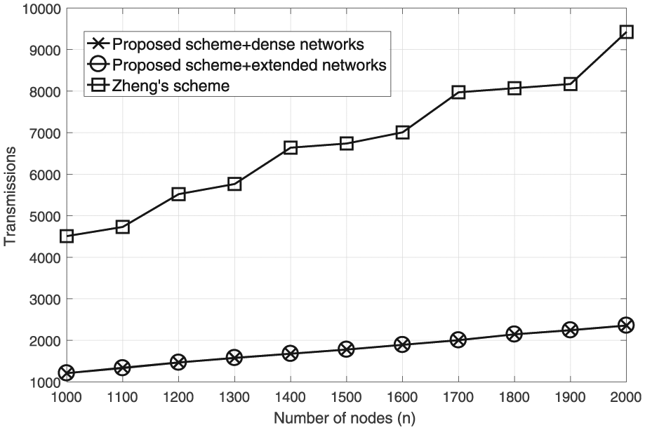
Next, we compare the total number of transmissions in the network, which is related to energy consumption and traffic loads in the network. We compare the proposed scheme to Zheng’s scheme. ⁹ Figure 8 compares the number of transmissions against $n$ . In Figure 8, we set the sparsity of constant order; we let $k=10$ . In addition, we set the communication range $r(n)=\sqrt{15\log n/n}$ and $r(n)=\sqrt{15\log n}$ for the dense and extended network models, respectively. In this simulation, dense and extended networks are defined as follows. In dense networks, the network area is fixed, and the number of nodes is increased. In extended networks, node density is fixed, and the network area is increased. For Zheng’s scheme, we use the dense network model. ⁹ Here, the number of transmissions of our scheme under the dense and extended network models is approximately equal because for a fixed number of nodes, the network topology is similar even under different scaling methods. Furthermore, we observe that the number of transmissions under our scheme is significantly smaller than that under Zheng’s scheme because in Zheng’s scheme, the heads in the cells construct the network backbone. Non-backbone nodes send raw data to heads, and the cell heads then relay data to the sink following the CDG method. Thus, the size of the backbone is exactly the number of cells in the network. However, in the proposed scheme, the backbone size is considerably smaller because our scheme finds the CDS from the network graph, which changes with node distribution. Thus, it is likely that our scheme will construct a small backbone adapted to the given network topology. However, the topology of the backbone is fixed in Zheng’s scheme; thus, it cannot adapt routing to a changing topology. This clearly shows the advantage of our graph-theoretic approach compared to that based on a network area with specific geometry. Alternatively, by applying an inequality similar to equation (12) to dense networks, the CDS size (backbone) is $O(r^{-2})=O(n/\log n)$ under our scheme, whereas that for Zheng’s scheme, it is $\Theta (n/\log n)$ . In other words, our backbone size is asymptotically no larger than that of Zheng’s scheme.

Figure 8.

Comparison of number of transmissions with varying $n$ .

Figure 9 compares the total energy consumption of the proposed scheme and Zheng’s scheme. In Figure 9, we set path loss constant $\alpha =3$ , ambient noise power $N_0=-30\mathrm{dBm}$ , SINR threshold $\eta =30\mathrm{dB}$ , constant $c_2=2$ , and RX $P_r=-10\mathrm{dBm}$ . Under the dense network model, the energy consumption of our scheme is less than that of Zheng’s scheme because the total number of transmissions of the proposed scheme is less than that of Zheng’s scheme. Moreover, the energy consumption under the extended network is considerably greater than that under the dense network because the communication range under the extended network model is greater than that under the dense network model by a factor of $\sqrt{n}$ . Another observation is that the rate of increase in energy consumption is small for large $n$ under the dense network model because as $n$ tends to infinity, TX power vanishes; thus, the RX power dominates energy consumption.

Figure 9.

Comparison of energy consumption with varying $n$ .

In the previous sections, we claimed the order-optimality of energy consumption when $k=O(1)$ . In this section, we numerically evaluate energy performance when sparsity $k$ is not $O(1)$ . Figure 10 compares the total energy consumption of the proposed scheme and Zheng’s scheme with sparsity $k=10\log n$ . The other parameters are the same as those in Figure 9. Similar to Figure 9, the energy consumption of our scheme is significantly less than that of Zheng’s scheme under the dense network model. Furthermore, under the dense network model, the gap between our scheme and Zheng’s scheme in Figure 10 $(k=\Theta (\log n))$ is even greater than that shown in Figure 9 $(k=\Theta (1))$ , which implies that the proposed scheme performs better with greater sparsity. This can be explained as follows. For fixed $n$ , sparsity $k$ in Figure 10 is greater than that in Figure 9. Greater sparsity implies a greater number of measurements because $m\propto k$ . Let $B_1$ and $B_2$ denote the backbone size of our scheme and Zheng’s scheme, respectively. The total number of transmissions over the backbone is approximately $m{B}_1$ (resp. $m{B}_2$ ) for our scheme (resp. Zheng’s scheme). Thus, the difference in the number of transmissions is approximately $m(B_2-B_1)$ . Previously, we argued that the backbone size in our scheme is smaller than that of Zheng’s; thus, the gap in the number of transmissions increases with increasing $m$ , which can be observed by comparing Figures 9 and 10. In conclusion, when sparsity $k$ grows faster than $O(1)$ , the proposed scheme is likely to perform even better due to the construction of efficient backbone networks.

Figure 10.

Comparison of energy consumption with sparsity $k=10\log n$ .

Conclusion and future work

In this article, we have proposed a joint routing and scheduling scheme for data collection that leverages hybrid CS. The proposed scheme is based on a graph-theoretical framework; thus, it is applicable to networks of arbitrary shape and topology. We constructed a CDS that serves as a network backbone and aggregated linearly combined data over the CDS in a pipelined manner. By properly setting the transmission range and backbone size, we demonstrated that the proposed scheme achieves order-optimal latency and low-energy consumption. Simulation results show that our scheme outperforms existing schemes in finite-size networks. In the future, we plan to integrate our protocol with practical packet reception methods based on PhIM. The packet-level PhIM (or packet reception ratio (PRR) versus SINR (SINR-PRR)) models the packet error rate as a function of SINR; thus, the SINR threshold $\eta$ in equation (5) determines the target PRR. However, there may exist significant variations in the measured SINR in large-scale WSNs. To address this issue, we may apply techniques based on the spatiotemporal diversity of traffic ²⁵ or regression-based modeling ²⁶ to our protocol to address fluctuations in the actual SINR and reduce measurement overhead.