Sage Journals: Discover world-class research

Abstract

Silent and autonomous work drives embedded systems to closely connect human on daily life. Recently, more and more embedded systems join service chain to form greatly embedded networks. In addition, low-cost and speed time-to-market characteristics make the increase in embedded network being exponential. As a result, a new battleground of energy saving become a significant challenge as a huge amount of embedded systems collaborate with tasks. To combat energy consumption, we propose an energy-aware path strategy to achieve energy saving. It is designed for system level so as to early examine energy utilization. Our contribution focuses on modeling-embedded network by path matrix. Improving energy evaluation takes dynamic and static energy into consideration. Presenting a new approach on energy distribution evolves from XY coordination to circle domain. The advantages consist of fast modeling various paths and calculating energy consumption. The effectiveness of the proposed method is verified by a set of benchmarks, and the results achieve energy saving for intricacy path of embedded networks.

Keywords

Energy-aware path strategy energy efficient embedded network embedded system task graph

Introduction

Embedded network is burdening power resource and energy cost. It is observed on the great growth of wireless networks, smartphones, and wearable devices. Widespread embedded systems with wireless network elements provide excellent quality of service resulting in the increase in energy consumption. In addition, mixed-criticality functions such as camera, camcorder, and MP3 player reside in embedded system to exhaust the energy capacity. Similarly, physiological signal monitoring of wearable devices exposes the efficient energy problem.

To improve energy efficiency of embedded systems, some researchers dedicate themselves into energy saving. The topics are cover component level, processor level, task level, and system level. On component level, Silva-Filho and Lima¹ addressed that memory hierarch consume microprocessor system powers up to 50%. They presented both the design flow and automated architecture exploration mechanism to reduce 27% energy consumption on MiBench and XiRisc suite experiments. From the viewpoint of processor level, Vilcu² studied real-time scheduling theory of CPU power consumption. He adapted CPU speed to improve power consumption. For task level, Fan et al.^3–5 presented model analysis, task allocation, and energy exploration technology to achieve energy efficiency. Moreover, Zeng et al.⁶ proposed combined dynamic level (CBL) algorithm that has over 25% improvement with comparison to existing list of scheduling heuristics. With consideration system level, Zeng et al.⁷ designed a software-centric framework called dynamic energy performance scaling that implemented dynamic hardware resource configuration (DHRC), dynamic voltage frequency scaling (DVFS), and dynamic power management (DPM) technologies to obtain the maximum energy savings. Furthermore, Park et al.⁸ proposed a fractional linear programming approach to multi-resource embedded systems. The synergy effect completed their objective in terms of energy efficiency.

Path theory is another valuable method on energy saving issue. The foremost effect is associated with critical path that is prior to the other paths. Therefore, Liu et al.⁹ presented low-energy static and dynamic scheduling algorithms based on critical-path analysis. Their approach evolved toward low-computational complexities. The energy saving of simulation results was up to 25% and 2% in dynamic and static scheduling algorithms, respectively. In 2013, a technical report by Ali et al.¹⁰ presented critical-path-first (CPF) heuristic algorithm on two-dimensional (2D) mesh multi-core processors. The critical path was associated with the highest impact on the execution time. Due to the reason that the work is getting more and more complex than before, the study of the number of paths is from single to multiple paths. Chang et al.¹¹ proposed trace-path analysis for multiple execution paths. It is helpful for multimedia-embedded system of performance estimation.

Problem description

An electronic device has embedded system to control other tasks for serving particular functions and providing more services than original system. Such architecture indicates that embedded system will seamlessly control the other tasks and then forms embedded networks. Therefore, we model the embedded system and a set of tasks as a root node and child nodes of task graph (TG) as tree. In addition, the tasks may also play roles as parents, siblings and descendant in tree. Each task is connected by the arc for the dependence and communication between two tasks.

Either embedded system or tasks consume energy whenever they run or are in sleep state. Two well-known energy consumptions are called dynamic and static energy dissipation that happen during working, sleeping, or leakage state.^3–5 Dynamic energy and static energy were consumed from embedded system to a number of tasks. However, neither one nor two paths link from embedded system to execute tasks. Inappropriately traversing path exacerbates more energy consumption. However, the leakage of transistors causes static energy consumption. Therefore, Patterson and Hennessy¹² stated that about 40% power consumption results from leakage. It indicates obviously that static energy caused from leakage is precious. As a result, well-arranged embedded network can improve energy consumption efficiently.

Based on the above discussion, the problem of energy consumption for embedded network is defined as follows. Given an embedded network which can be represented as tree structure, the objective is to improve energy consumption via energy-aware path strategy (EAPS).

EAPS

Embedded microcontroller

When designing embedded systems, microcontroller is usually seen as one of the essential components. It integrates necessary functions into a chip that comprises CPU core, program memory, data memory, data electrically erasable programmable read-only memory (EEPROM), and input/output peripheral. The iSuppli investigates the microcontroller market trend, which is presented in Table 1. Not only 8-bit microcontroller but also 32-bit microcontroller continues growth which is shown in the column of compound annual growth rate (CAGR).

Table 1.

Semiconductor MCU revenue market forecast—millions of dollars (courtesy of iSuppli¹³).

	2012	2013	2014	2015	2016	2017	CAGR (%)
Total semiconductor	325,367	339,666	361,612	385,052	395,974	413,602	4.9
Microcontroller (MCU)	16,008	16,202	17,211	18,799	19,307	20,480	5.1
4-Bit MCU	154	159	161	157	145	133	–2.8
8-Bit MCU	6057	6565	6936	7532	7768	8259	6.4%
16-Bit MCU	4021	3611	3765	4060	4053	4019	0.0%
32-Bit MCU	5776	5868	6349	7050	7341	8069	6.9%

CAGR: compound annual growth rate.

Embedded networks

Collaborative embedded system with many tasks is emerging in diversity embedded networks such as JPEG encoding system⁴ and adaptive pulse code modulation system (ADPCM).¹⁴ Both of them apply TG to model an evaluated system. TG is a conceptual graph that comprised vertices, edges, and levels. The vertices are also called nodes which are used to represent task. The edge is used to point the flow of node. Each edge links two nodes. For example, an edge communicates node X to node Y, which depicts the control flow from task X to task Y. The level is used to denote the height of evaluating system.

Figure 1 shows one of the evaluated embedded networks which consisted of 8 nodes and 10 edges. Thus, two sets will be created while the evaluated network is given. One set is related to node N = {n₀, n₁, n₂, …, n₇}. The other set is associated of edge A = {a₀, a₁, …, a₉}. Another element is the height of tree as 4. In consideration of embedded network cooperates with other tasks. As embedded system as the role of controller, it is assigned as root as node id 0. It can communicate to other tasks such as node id 1, 2, 3 and 4 via a subset of edge.

Figure 1.

Embedded network with eight nodes.

Path matrix

Given an arbitrary embedded network such as Figure 2(a), a set of path will be constructed which is depicted in Figure 2(b)–(f). The first path is demonstrated in Figure 2(b) which is departed from root and pass by node id 1, 5, and 7. It is a classic case in network topology because of routing adjacent level. It is named P_a. Path id 0, p₀, is defined as P_a = {0, 1, 5, 7} in path matrix. The second path starts from root and visits node id 2 and 7 in Figure 2(c). From the tour-level point of view, it is different from p₀. It routes through adjacent and explicit cross levels and denoted as P_ac. In path matrix, it is expressed as p₁ = {0, 2, 7}. The third path is shown in Figure 2(d) that starts from the node id 0 to next stop by crossing two levels. We define it as P_cx, where suffix x is used to point the number of crossing. It is expressed as p₂ = {0,7} as path matrix. The fourth path is as same as P_ac. The path class is expressed as p₃ = {0, 3, 7}. The fifth path is marked P_ci, where routes through adjacent and implicitly cross levels. The segment of path from node ids 4 to 7 happens implicitly in cross levels. Its trip includes node id 4 and 7 rather than node id 4, 6, or 7. The path matrix is expressed as p₄ = {0, 4, 7}.

Figure 2.

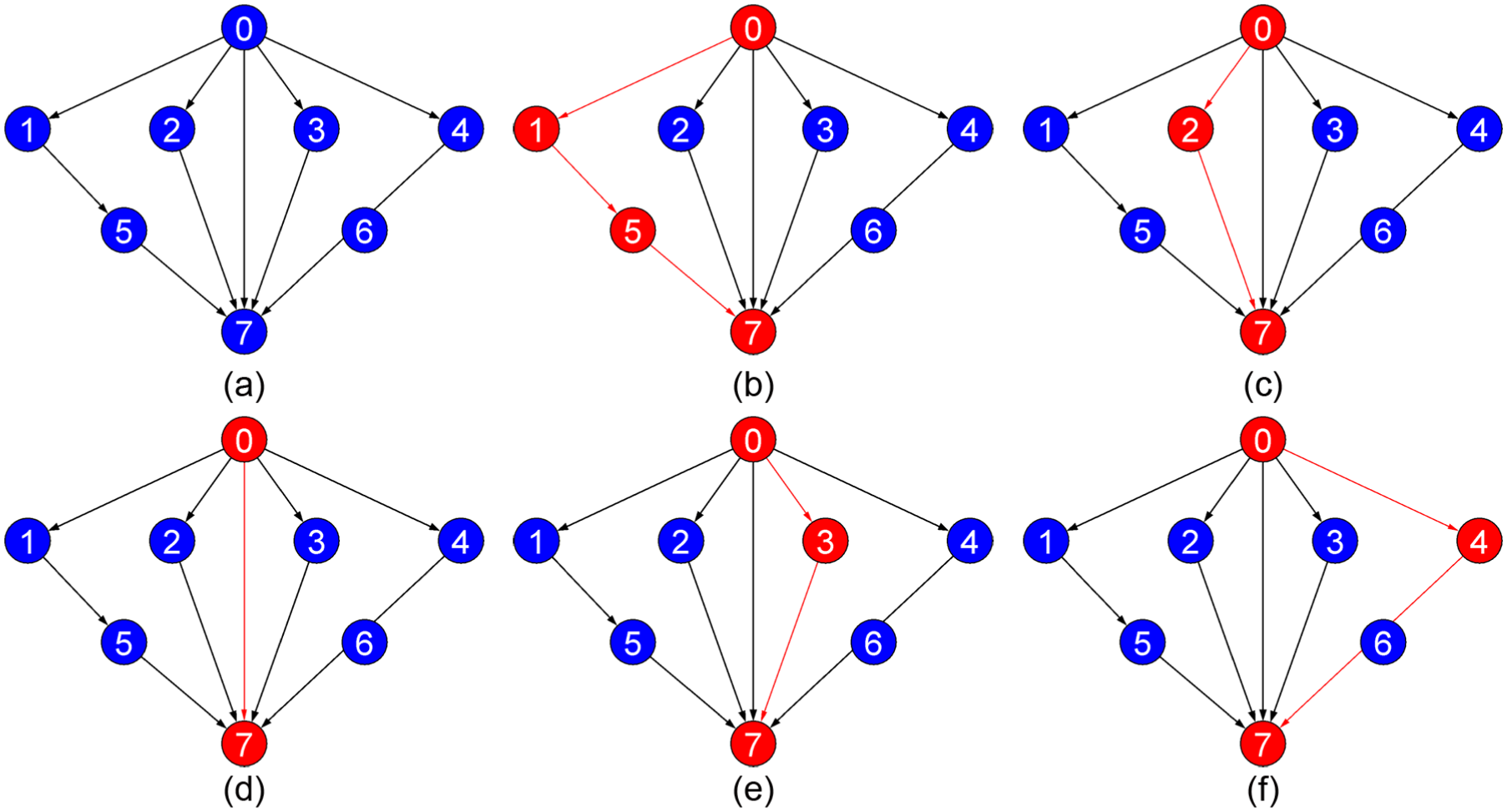
(a) Embedded network with eight nodes. (b) The first path routes through adjacent levels. (c) The second path routes through adjacent and explicit cross levels. (d) The third path routes through explicit two cross levels. (e) The fourth path routes through adjacent and explicit cross levels. (f) The fifth path routes through adjacent and implicit cross levels.

According to previous state, the path matrix is defined in the following

\begin{matrix} \begin{matrix} 0 & 1 & 2 & 3 & 4 \end{matrix} \\ \begin{matrix} 0 \\ 1 \\ 2 \\ 3 \\ 4 \\ 5 \\ 6 \\ 7 \end{matrix} (\begin{matrix} 1 & 1 & 1 & 1 & 1 \\ 1 & 0 & 0 & 0 & 0 \\ 0 & 1 & 0 & 0 & 0 \\ 0 & 0 & 0 & 1 & 0 \\ 0 & 0 & 0 & 0 & 1 \\ 1 & 0 & 0 & 0 & 0 \\ 0 & 0 & 0 & 0 & 0 \\ 1 & 1 & 1 & 1 & 1 \end{matrix}) \end{matrix}

(1)

where rows represent the number of nodes and the columns represent the number of paths. Equation (1) shows the path matrix that needs further to find the energy saving architecture of embedded node.

EAPS

Electric energy is defined as the electrical power P multiply executing time T. Inside embedded systems, there are two aspects of power consumed. One is dynamic power and the other is static power. Both dynamic and static power affects the design consuming the energy quantity. Regarding of dynamic power, it is associated with the power consumption on executing task while the node is working. On the other hand, the static power consumes energy results from the leakage of transistors. Therefore, the dynamic energy consumption, E_d, and static energy consumption, E_s, are defined as follows

E_{d} = P_{d} \times T_{d}

(2)

E_{s} = P_{s} \times T_{s}

(3)

where subscript d and s represents dynamic and static power, respectively.

For a given embedded network shown in Figure 2(a), we model dynamic and static energy consumption as mirror structure that is displayed in Figure 3. On one hand, the embedded network consumes dynamic energy consumption E_d. On the other hand, the system consumes static energy consumption.

Figure 3.

Mirror structure of dynamic and static energy for embedded network.

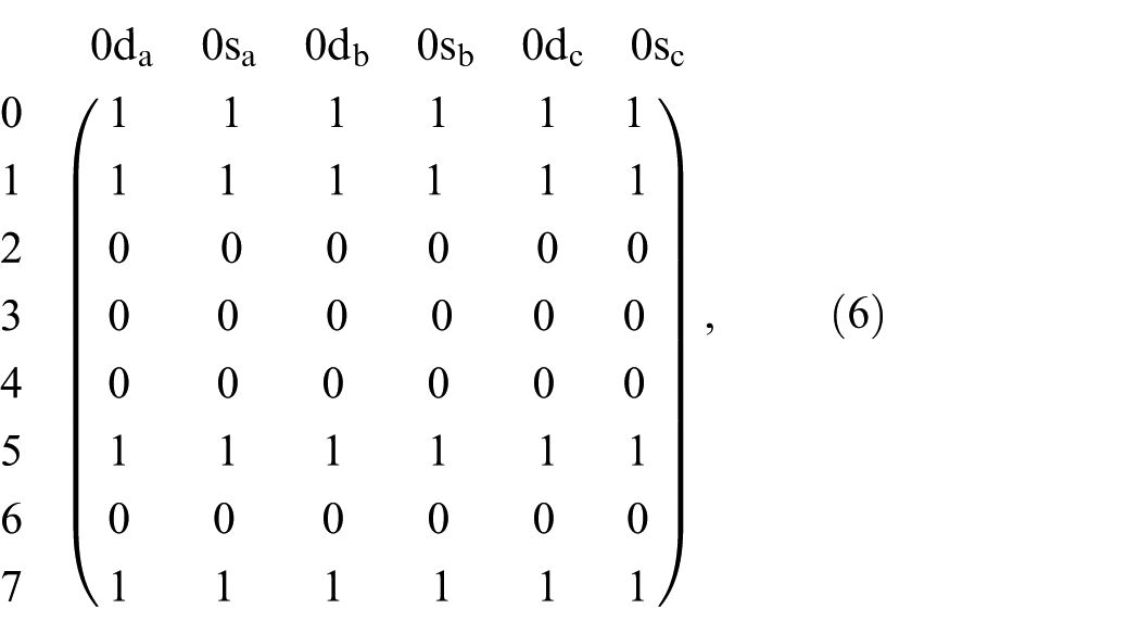
Depending on the Figure 3 with mirror characteristic, the dynamic and static energy consumption of path id 0 are arranged in the same rows and then denote it in the following

\begin{matrix} \begin{matrix} 0 d & 0 s \end{matrix} \\ \begin{matrix} 0 \\ 1 \\ 2 \\ 3 \\ 4 \\ 5 \\ 6 \\ 7 \end{matrix} (\begin{matrix} 1 & 1 \\ 1 & 1 \\ 0 & 0 \\ 0 & 0 \\ 0 & 0 \\ 1 & 1 \\ 0 & 0 \\ 1 & 1 \end{matrix}) \end{matrix}

(4)

where the column “0d” represents the dynamic energy consumption shown in the left side of Figure 3 and the other column “0s” represents static energy consumption shown in right side.

To explore the energy distribution taking into account Figure 3 with equation (4), both dynamic and static energy are transformed to XY domain that is illustrated in Figure 4.

Figure 4.

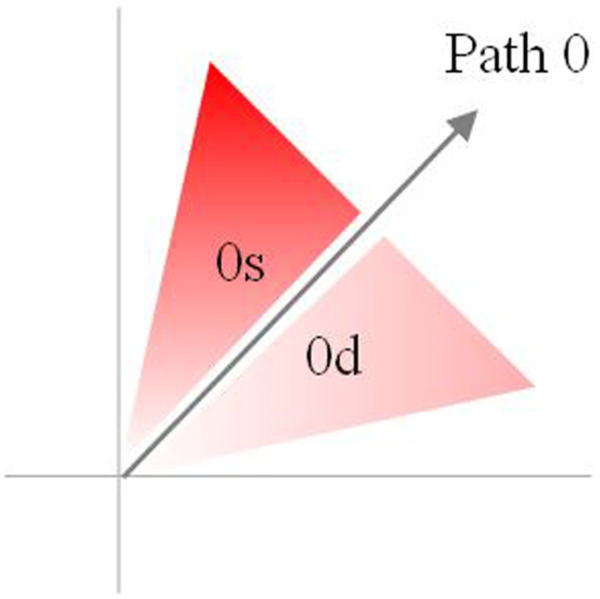
Energy distribution of one path for path id 0.

However, not only one route but also two routes are deployed in embedded networks. Hence, it can be a formula for two routes in the following

\begin{matrix} \begin{matrix} 0 d_{a} & 0 s_{a} & 0 d_{b} & 0 s_{b} \end{matrix} \\ \begin{matrix} 0 \\ 1 \\ 2 \\ 3 \\ 4 \\ 5 \\ 6 \\ 7 \end{matrix} (\begin{matrix} 1 & 1 & 1 & 1 \\ 1 & 1 & 1 & 1 \\ 0 & 0 & 0 & 0 \\ 0 & 0 & 0 & 0 \\ 0 & 0 & 0 & 0 \\ 1 & 1 & 1 & 1 \\ 0 & 0 & 0 & 0 \\ 1 & 1 & 1 & 1 \end{matrix}) \end{matrix},

(5)

where subscript “a” of the columns “0d_a” and “0s_a” indicates the one route and the other subscript “b” of columns “0d_b” and “0s_b” is represented as the second route. Their energy distribution of XY domain is demonstrated in Figure 5.

Figure 5.

Energy distribution of two paths for path id 1.

Similarly, it can be the following formula if path id 0 has three routes

\begin{matrix} \begin{matrix} 0 d_{a} & 0 s_{a} & 0 d_{b} & 0 s_{b} & 0 d_{c} & 0 s_{c} \end{matrix} \\ \begin{matrix} 0 \\ 1 \\ 2 \\ 3 \\ 4 \\ 5 \\ 6 \\ 7 \end{matrix} (\begin{matrix} 1 & 1 & 1 & 1 & 1 & 1 \\ 1 & 1 & 1 & 1 & 1 & 1 \\ 0 & 0 & 0 & 0 & 0 & 0 \\ 0 & 0 & 0 & 0 & 0 & 0 \\ 0 & 0 & 0 & 0 & 0 & 0 \\ 1 & 1 & 1 & 1 & 1 & 1 \\ 0 & 0 & 0 & 0 & 0 & 0 \\ 1 & 1 & 1 & 1 & 1 & 1 \end{matrix}) \end{matrix},

(6)

where subscript “c” of columns “0d_c” and “0s_c” represent the third route.

Their energy distribution is shown in Figure 6(a). Based on the same rule, the four routes of energy distribution can be derived in Figure 6(b). Figure 7 demonstrates the energy-aware traversal process of path id 0 with one route. To achieve it, the first step is, to obtain the dynamic and static energy consumption investigates from the specification for each node. Either electronic dynamic power P_d or electronic static power P_s is essential. Based on equations (2) and (3), both dynamic and static energy consumption are calculated by electronic power P and execution time T. For this reason, we collect separately execution time T_d and T_s for each node so as to construct two sets of energy consumption. Figure 7(a) demonstrates the two sets of energy consumption for each node. One is associated with dynamic energy consumption E_d and the other corresponded to static energy dissipation E_s. Second, according to path equation (4), we take the first path, path id 0, to calculate the energy consumption that is exhibited in Figure 7(b). Considering that the embedded network plays a role in controlling other tasks, the node id 0 is set as embedded system resulting in the calculating process from top to bottom. Besides, an element consumes dynamic energy accompanying with static energy dissipation resulting from other elements’ leakage. These phenomena are shown in Figure 7(c) and (d). The former presents separately embedded system and node id 1 consume dynamic energy which is labeled as “0d_a0” and “0d_a1”. Other tasks such as (1, 5, 7) and (0, 5, 7) simultaneously consume static energy which is separately accompanied with node ids 0 and 1. It is easily analyzed for the energy consumption for different elements in path. On the contrary, the latter demonstrates dynamic energy dissipation for the other elements that is referenced as “0d_a2” and “0d_a3.” Other paths will be calculated sequentially if the number of paths is more than one. After complete calculation of energy consumption for all paths, the energy-aware path with a minimum energy consumption of embedded network is obtained in Figure 7(e).

Figure 6.

(a) Energy distribution of three paths for path id 0 and (b) energy distribution of four paths for path id 0.

Figure 7.

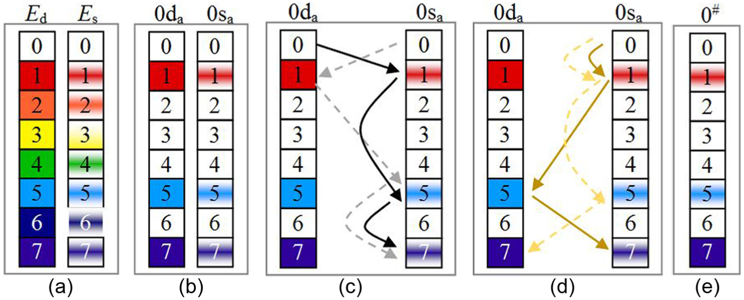
(a) Energy consumed for embedded node with one route, (b) dynamic and static energy consumed for path id 0, (c) calculation of energy consumption via dynamic energy for nodes 0 and 1, (d) calculation of energy consumption via dynamic energy for nodes 5 and 7, and (e) result of energy-aware traversal.

Not only one but also more paths flow from embedded system to other tasks. Each branch separately consumes out of control energy. In order to improve energy consumption, well-manipulating branch is proposed in this work from hundreds of thousands pipes. To facilitate evaluation of energy consumed for each path, we transform energy consumption from XY domain to circle domain.

Figure 8 exhibits energy consumption by circle domain. First, Figure 8(a) shows the energy distribution for the one path. The “0d_a” and “0s_a” energy distribution locate between 0°–45° and 45°–90°, respectively. Therefore, the energy dissipation can be assessed on one of fourth circle by equation (7). Second, in consideration of embedded network have two paths. Their energy distribution will separately arrange on 0 to 90 and 90 to 180 degree that is depicted in Figure 8(b) and Figure 8(c). For “0d_a” in Path 0_a, it consumes static energy either “0s_a” and “0s_b.” On the contrary, the “0d_b” of path 0_b consumes static energy either “0s_a” or “0s_b.” Thus, it forms two routes either “0d_a” or “0d_b” and their energy consumption can be calculated by equation (8). According to Figure 8(a)–(c), we conclude that the energy distribution is shown in Figure 8(d). Both of them can apply to any number of paths which are displayed in Figure 8(e) and equation (9).

Figure 8.

Energy consumption in circle domain: (a) energy distribution for the one path, (b) energy distribution on 0 to 90 degree, (c) energy distribution on 90 to 180 degree, (d) normalize energy distribution for one path, and (e) normalize energy distribution for any number of paths.

E_{i} \times \frac{45 \circ}{360 \circ} + E_{j} \times \frac{45 \circ}{360 \circ}

(7)

where i ≠ j, i and j represent dynamic and static energy consumption for one path, respectively

\sum_{i} E_{i} \times \frac{45 \circ}{360 \circ} + i \times \sum_{j} [E_{j} \times \frac{45 \circ}{360 \circ} \times α_{j}]

(8)

where i ≠ j, {i, j, α} = 1, 2, 3…, n, $n \in N$ , and α is the path id of static energy consumption

\sum_{i} E_{i} \times \frac{θ_{u}}{360 \circ} + i \times \sum_{j} [E_{j} \times \frac{θ_{v}}{360 \circ} \times α_{j}]

(9)

where u = v, i ≠ j, {i, j, α} = 1, 2, 3…, n, $n \in N$ , and u and v are the angle of energy distribution.

Experimental results and analysis

The proposed EAPS was implemented in Java programming language and executed on a Windows machine with a 3.2 GHz i5-4570 processor and 4 GB memory. This work conducted the experiments on the four sets, A, B, C and D, of TGFF^15–17 benchmarks. Each set consisted of six benchmarks: (1) M series (100 tasks), (2) L series (150 tasks), (3) V series (200 tasks), (4) U series (250 tasks), (5) W series (300 tasks), and (6) X series (350 tasks). Each series is simulated with four kinds of set. The column “Nodes” represents the number of nodes that is one specification for constructing test case. “Cand.” denotes the number of candidates in simulating process. It is apparently double larger than the "Nodes" because of equation (5). That is, each node allocates two candidates which consume different energy.“Level” represents the height of tree for creating benchmark. The column “Nodes in each levels” show the number of tasks in each level. The column “Paths” displays the quantity of paths for each benchmarks. The experimental information for all benchmarks are listed in Table 2.

Table 2.

Applications in each class-related information of benchmarks.

Benchmarks		Nodes	Cand.	Levels	Nodes in each levels	Paths
A	M₁	100	200	10	(1, 10, 12, 11, 12, 13, 14, 12, 14, 1)	206
	L₁	150	300		(1, 19, 21, 17, 18, 21, 22, 14, 16, 1)	935
	V₁	200	400		(1, 23, 22, 24, 23, 29, 32, 23, 22, 1)	4878
	U₁	250	500		(1, 28, 26, 35, 26, 30, 32, 34, 37, 1)	11,680
	W₁	300	600		(1, 38, 29, 36, 36, 51, 37, 35, 36, 1)	40,036
	X₁	350	700		(1, 37, 46, 53, 39, 54, 37, 43, 39, 1)	101,753
B	M₂	100	200	15	(1, 7, 5, 6, 9, 8, 5, 10, 9, 7, 9, 5, 12, 6, 1)	314
	L₂	150	300		(1, 12, 6, 5, 8, 9, 14, 11, 9, 9, 17, 17, 17, 14, 1)	1623
	V₂	200	400		(1, 20, 19, 18, 18, 16, 12, 15, 14, 9, 18, 8, 16, 15, 1)	8792
	U₂	250	500		1, 22, 21, 27, 20, 21, 18, 18, 24, 17, 10, 18, 18, 14, 1	17,321
	W₂	300	600		(1, 29, 21, 24, 14, 24, 32, 15, 19, 25, 20, 15, 28, 32, 1)	94,558
	X₂	350	700		(1, 26, 22, 30, 27, 23, 25, 31, 32, 38, 20, 21, 27, 26, 1)	394,824
C	M₃	100	200	20	(1, 5, 5, 6, 11, 5, 10, 10, 6, 8, 3, 2, 2, 2, 4, 6, 4, 5, 4, 1)	336
	L₃	150	300		(1, 12, 8, 10, 9, 8, 7, 10, 7, 7, 11, 7, 7, 5, 7, 11, 6, 10, 6, 1)	1995
	V₃	200	400		(1, 7, 11, 13, 9, 13, 14, 12, 13, 4, 14, 14, 6, 10, 10, 17, 7, 11, 13, 1)	7744
	U ₃	250	500		(1, 10, 13, 11, 16, 9, 13, 8, 12, 19, 14, 16, 12, 23, 18, 11, 12, 16, 15, 1)	57,643
	W₃	300	600		(1, 14, 15, 14, 17, 14, 22, 18, 16, 15, 15, 17, 26, 8, 17, 19, 19, 15, 17, 1)	225,858
	X₃	350	700		(1, 21, 22, 20, 21, 13, 17, 21, 24, 19, 16, 20, 26, 20, 19, 17, 23, 16, 13,1)	726,931
D	M₄	100	200	25	(1, 3, 4, 3, 9, 4, 6, 4, 3, 4, 5, 3, 5, 5, 4, 3, 5, 1, 3, 2, 4, 10, 3, 5, 1)	385
	L₄	150	300		(1, 4, 8, 8, 7, 8, 5, 6, 7, 13, 6, 7, 6, 8, 7, 3, 6, 4, 5, 7, 5, 3, 7, 8, 1)	2691
	V₄	200	400		(1, 12, 11, 11, 8, 7, 6, 12, 6, 9, 7, 10, 5, 7, 11, 14, 7, 14, 8, 8, 7, 8, 5, 5, 1)	11,454
	U₄	250	500		(1, 16, 11, 9, 11, 8, 9, 7, 15, 5, 14, 7, 11, 11, 13, 12, 10, 15, 12, 6, 12, 8, 13, 13, 1)	90,164
	W₄	300	600		(1, 9, 12, 16, 13, 11, 15, 10, 15, 9, 13, 16, 13, 15, 10, 20, 13, 15, 12, 13, 15, 8, 14, 11, 1)	369,598
	X₄	350	700		(1, 12, 9, 19, 16, 17, 12, 22, 13, 12, 14, 17, 15, 14, 8, 14, 19, 13, 9, 19, 16, 22, 21, 15, 1)	1,355,438

In the experiments, we perform the proposed EAPS to A, B, C, and D sets. Figure 9 exhibits the flowchart of experiments. First, we generate random benchmark of embedded networks according to the number of nodes and levels that are given by designer. Thus, an embedded network will be created that is consisted of the number of nodes and arcs. The graph nodes are used to simulate tasks and the arcs are used to represent the routes. Second, we produce randomly a set of energy parameter d that is associated with nodes. The elements d₁, d₂, …, d_m of d will be used to calculate energy dissipation. After that, the EAPS is applied to benchmarks to achieve minimum energy dissipation. It begins from analyzing architecture of benchmark and then arranging as a set of path P. Each subset p₁, p₂, …, p_n of P will be evaluated for energy consumption. However, there are diversity candidates who reside in the candidate column. Consequently, we arrange a subset of nodes N_x that is included in a set of node N. Next, we analyze each possible combination N_y and then calculate their energy dissipation. Each subset N_y₁, N_y2, …, N_yt consumes energy derived from energy dissipation set S. Finally, the least energy consumption is filtered from the subset node N_z. The rest of paths are performed the previous steps until the last path is analyzed.

Figure 9.

Flow chart of experiment.

Figure 10 shows X₄ benchmarks in D set. The EAPS arranges path set P = {p₀, p₁, …, p_1355437} according to the X₄ architecture. Thus, there are over one million paths will be analyzed by EAPS. Table 3 shows the travel information for some paths. The first path, p₀, routes nodes 0 and 2. The candidate subset consumes maximum and minimum energy of 6.33 × 10⁻⁴ and 3.58 × 10⁻⁴, respectively. Thus, the node set with minimum energy will be set. Another path id 339 consumes maximum and minimum energy of 0.013 and 0.006, respectively. Thus, the pop subset nodes N_z ={0111011111111} are determined by the traveling nodes {0-17-58-139-148-171-197-222-256-280-298-325-349}, which demonstrates the red color path in Figure 10. The other path id 1340647 follows the same rule.

Figure 10.

X4 benchmark.

Table 3.

Routing table for X4 benchmark.

Path id	Traveling nodes	Maximum energy consumed	Minimum energy consumed
0	0–2	6.33 × 10⁻⁴	3.58×10⁻⁴
339	0-17-58-139-148-171-197-222-256-280-298-325-349	0.013	0.006
134,0647	50-75-94-115-124-181-196-230-256-280-298-325-349	0.012	0.005

Table 4 presents the experimental results of energy dissipation for comparison of heuristic approach and EAPS approach. Each benchmark is executed 15 times with heuristic approach. Figure 11 demonstrates the algorithm of heuristic approach. For a given embedded network with a set of nodes N and the number of height H, the heuristic algorithm can calculate the energy consumption E. First, the nodes are randomly set for each path (line 1). Then, to calculate the energy consumption for each level (line 6), energy dissipation is derived. Next, to compute the dynamic energy E_d in one level (line 7–8) and static energy E_s in the other levels (line 9–10), energy consumption for specific level was collected. After all levels are quantified, the energy dissipation is measured by sum of E_d and E_s (line 12). For example, the first path, p₀, for r₁ are first randomly set N_z = {1,0} but EAPS sets N_z = {0,0}. Another path, p₃₃₉, is arbitrarily set N_z = {1011011001110} in comparison with EAPS as N_z = {0111011111111}. The other path, p₃₄₀, is traveling nodes as {0-17-58-139-148-171-197-222-256-280-298-332-340} that the nodes are randomly set to N_z = {1011011001100}. In contrast, the EAPS obtains N_z = {0111011111111}. After all nodes of all paths are set, the new set called new_N (line 1) is generated. Then, the rest of procedures of heuristic algorithm calculate the energy dissipations. Other benchmarks from r₂ to r₁₅ consume energy to adhere to procedures of r₁. Their energy dissipations are displayed in the column from r₁ to r₁₅. The column, “Imp,” is defined as (1 − EAPS/(sum(r₁:r₁₅)/15)) × 100. For “Avg,” it is defined as sum(Imp)/24. It indicates that EAPS takes 35.98% improvement than heuristic approach.

Table 4.

Comparison for energy dissipation with heuristic approach and EAP algorithm.

	Energy dissipation																%
Heuristic																Our	Imp.
	r ₁	r ₂	r ₃	r ₄	r ₅	r ₆	r ₇	r ₈	r ₉	r ₁₀	r ₁₁	r ₁₂	r ₁₃	r ₁₄	r ₁₅	Our	Imp.
M ₁	0.132	0.140	0.143	0.135	0.146	0.139	0.136	0.150	0.143	0.134	0.145	0.137	0.152	0.147	0.148	0.120	15.37
L ₁	0.063	0.082	0.092	0.067	0.076	0.087	0.086	0.084	0.106	0.086	0.089	0.078	0.087	0.090	0.078	0.012	85.61
V ₁	0.094	0.099	0.102	0.104	0.097	0.096	0.101	0.103	0.095	0.100	0.093	0.097	0.102	0.105	0.093	0.068	31.13
U ₁	0.229	0.231	0.235	0.237	0.239	0.236	0.234	0.231	0.234	0.243	0.248	0.228	0.227	0.239	0.228	0.227	3.24
W ₁	0.378	0.390	0.387	0.367	0.365	0.363	0.382	0.376	0.374	0.380	0.385	0.371	0.389	0.377	0.391	0.327	13.57
X ₁	0.344	0.347	0.329	0.345	0.334	0.341	0.352	0.336	0.343	0.346	0.349	0.347	0.345	0.346	0.342	0.329	4.10
M ₂	0.119	0.117	0.109	0.122	0.118	0.113	0.111	0.106	0.111	0.104	0.116	0.123	0.117	0.108	0.102	0.086	23.94
L ₂	0.192	0.177	0.179	0.184	0.199	0.172	0.194	0.180	0.185	0.175	0.194	0.186	0.200	0.165	0.189	0.082	55.61
V ₂	0.421	0.413	0.413	0.411	0.444	0.410	0.424	0.412	0.404	0.420	0.412	0.418	0.407	0.423	0.413	0.372	10.65
U ₂	0.330	0.336	0.331	0.337	0.327	0.335	0.342	0.346	0.339	0.321	0.324	0.344	0.340	0.336	0.333	0.327	2.31
W ₂	0.511	0.572	0.531	0.601	0.517	0.560	0.553	0.548	0.540	0.516	0.546	0.563	0.569	0.541	0.538	0.279	49.00
X ₂	0.437	0.487	0.442	0.442	0.444	0.455	0.447	0.448	0.438	0.451	0.469	0.443	0.453	0.468	0.472	0.293	35.33
M ₃	0.121	0.110	0.109	0.133	0.113	0.130	0.135	0.139	0.097	0.133	0.109	0.104	0.114	0.153	0.112	0.026	78.48
L ₃	0.213	0.206	0.212	0.214	0.227	0.206	0.180	0.199	0.227	0.193	0.176	0.217	0.196	0.200	0.208	0.111	45.84
V ₃	0.564	0.591	0.576	0.614	0.587	0.544	0.554	0.600	0.534	0.562	0.602	0.541	0.625	0.627	0.575	0.156	73.09
U ₃	0.658	0.672	0.645	0.665	0.661	0.653	0.643	0.643	0.676	0.673	0.638	0.683	0.667	0.663	0.681	0.636	3.84
W ₃	0.194	0.191	0.189	0.192	0.200	0.185	0.194	0.194	0.182	0.181	0.192	0.191	0.200	0.190	0.205	0.139	27.60
X ₃	1.074	1.092	1.081	1.056	1.018	1.095	1.023	1.111	1.060	1.027	1.042	1.055	1.051	1.071	1.038	0.663	37.43
M ₄	0.150	0.140	0.143	0.132	0.152	0.139	0.154	0.121	0.153	0.149	0.132	0.154	0.156	0.146	0.144	0.074	48.73
L ₄	0.217	0.225	0.236	0.223	0.235	0.220	0.218	0.215	0.214	0.239	0.237	0.220	0.229	0.241	0.231	0.144	36.47
V ₄	0.460	0.473	0.403	0.474	0.476	0.431	0.452	0.438	0.486	0.462	0.459	0.409	0.496	0.456	0.417	0.167	63.12
U ₄	0.283	0.326	0.325	0.331	0.298	0.312	0.313	0.323	0.314	0.324	0.289	0.292	0.341	0.303	0.301	0.111	64.39
W ₄	0.706	0.727	0.707	0.709	0.714	0.702	0.712	0.693	0.715	0.706	0.716	0.708	0.694	0.715	0.707	0.622	12.24
X ₄	0.390	0.396	0.389	0.408	0.394	0.394	0.386	0.388	0.366	0.375	0.380	0.369	0.376	0.380	0.392	0.222	42.42
Avg.																	35.98

Figure 11.

Algorithm heuristic approach.

Conclusion

Energy saving is always a significant issue for electronic world. In this work, we present an EAPS to assess energy consumption of embedded networks in the early stage. We first model as embedded network a set of path matrix. With precise evaluation of energy dissipation, the dynamic and static energy consumption is involved in the energy effect. For emulating embedded networks, we elaborate energy distribution from XY domain to circle domain. Transforming into circle coordination gains easily modeling multiple paths and calculating energy. Finally, the proposed method is tested by a set of benchmarks and the experimental results have shown the effectiveness.

Footnotes

Acknowledgements

The author would like to thank the National Science Council of the Republic of China, Taiwan, for financially supporting this research under Contract No. NSC102-2221-E-143-002.

Handling Editor: Yudong Zhang

Declaration of conflicting interests

The author(s) declared no potential conflicts of interest with respect to the research, authorship, and/or publication of this article.

Funding

The author(s) received no financial support for the research, authorship, and/or publication of this article.

References

Silva-Filho

Lima

SML

. Energy consumption reduction mechanism by tuning cache configuration using NIOS II processor. In: Proceedings of the IEEE international SOC conference, Newport Beach, CA, 17–20 September 2008, pp.291–294. New York: IEEE.

Vilcu

Real time scheduling and CPU power consumption in embedded systems. In: IEEE international conference on automation, quality and testing, robotics, Cluj-Napoca, 22–25 May 2008, pp.261–266. New York: IEEE.

Fan

Wang

SF.

Low power dissipation model analysis for embedded systems. Res Not Inf Sci 2013; 13: 184–188.

Fan

Wang

SF.

Energy efficiency of task allocation for embedded JPEG systems. Sci World J 2014; 2014: 718348.

Fan

Wang

SF.

Efficient energy exploration for embedded systems. In: Proceedings of the 18th IEEE international symposium on consumer electronics, JeJu Island, South Korea, 22–25 June 2014, pp.324–325. New York: IEEE.

Zeng

Wei

Liu

Research of optimal task scheduling for distributed real-time embedded systems. In: Proceedings of the IEEE international conference on embedded software and systems, Sichuan, China, 29–31 July 2008, pp.77–84. New York: IEEE.

Zeng

Tomiyama

Takada

A generalized framework for system-wide energy savings in hard real-time embedded systems. In: Proceedings of the IEEE international conference on embedded and ubiquitous computing, Shanghai, China, 17–20 December 2008, pp.206–213. New York: IEEE.

Park

Raghunathan

Srivastava

MB.

Energy efficiency and fairness tradeoffs in multi-resource, multi-tasking embedded systems. In: Proceedings of the ACM 2003 international symposium on low power electronics and design, Seoul, South Korea, 27–27 August 2003, pp.469–474. New York: IEEE.

Liu

Veeravalli

Viswanathan

Novel critical-path based low-energy scheduling algorithms for heterogeneous multiprocessor real-time embedded systems. In: Proceedings of the IEEE international conference on parallel and distributed systems, Hsinchu, Taiwan, 5–7 December 2007, pp.1–8. New York: IEEE.

10.

Ali

Pinho

Akesson

Critical-path-first based allocation of real-time streaming applications on 2D mesh-type multi-cores. In: Proceedings of the 19th IEEE international conference on embedded and real-time computing systems and applications, Taipei, Taiwan, 19–21 August 2013, pp.201–208. New York: IEEE.

11.

Chang

Lee

Jen

CW.

Trace-path analysis and performance estimation for multimedia application in embedded system. In: Proceedings of the IEEE international symposium on circuits and systems, Vancouver, BC, Canada, 23–26 May 2004, pp.II–129–132. New York: IEEE.

12.

Patterson

Hennessy

. Computer organization and design: the hardware/software interface. 5th ed.

Elsevier

Taiwan, 2014, pp.42.

13.

Semiconductor MCU revenue market forecast—millions of dollars; courtesy of iSuppli, http://www.atmel.com/images/45107a-choosing-a-mcu-fredriksen_article_103114.pdf

14.

Lee

Fan

Cheng

et al . Hardware-software partitioning for embedded multiprocessor FPGA systems. Int J Innov Comput I 2009; 5(10A): 3071–3083.

15.

Dick

Rhodes

Wolf

TGFF: task graphs for free. In: Proceedings of the IEEE international workshop on hardware/software codesign, Seattle, WA, 18 March 1998, pp.97–101. New York: IEEE.

16.

Kwok

Ahmad

Benchmarking and comparison of the task graph scheduling algorithms. J Parallel Distr Com 1999; 59(3): 381–422.

17.

Vallerio

Jha

NK.

Task graph extraction for embedded system synthesis. In: Proceedings of the IEEE 16th international conference on VLSI design, New Delhi, India, 4–8 January 2003, pp.480–486. New York: IEEE.

Energy-aware path strategy for embedded network

Abstract

Keywords

Introduction

Problem description

EAPS

Embedded microcontroller

Embedded networks

Path matrix

EAPS

Experimental results and analysis

Conclusion

Footnotes

Acknowledgements

Declaration of conflicting interests

Funding

References