Characterizing user mobility using mobile sensing systems

Abstract

Recent technological advances and the ever-greater developments in sensing and computing continue to provide new ways of understanding our daily mobility. Smart devices such as smartphones or smartwatches can, for instance, provide an enhanced user experience based on different sets of built-in sensors that follow every user action and identify its environment. Monitoring solutions such as these, which are becoming more and more common, allows us to assess human behavior and movement at different levels. In this article, extended from previous work, we focus on the concept of human mobility and explore how we can exploit a dataset collected opportunistically from multiple participants. In particular, we study how the different sensor groups present in most commercial smart devices can be used to deliver mobility information and patterns. In addition to traditional motion sensors that are obviously important in this field, we are also exploring data from physiological and environmental sensors, including new ways of displaying, understanding, and analyzing data. Furthermore, we detail the need to use methods that respect the privacy of users and investigate the possibilities offered by network traces, including Wi-Fi and Bluetooth communication technologies. We finally offer a mobility assistant that can represent different user characteristics anonymously, based on a combination of Wi-Fi, activity data, and graph theory.

Introduction

The rapid emergence of new technologies and the continuing expansion of networks, both fixed and mobile, promise new possibilities for understanding human behavior. Whether in smartphones, smartwatches, or specialized equipment, the miniaturization of sensors and the popularity of these devices allow both industry and science to propose valuable new models, concepts, and prototypes. This network of sensors, also considered as a set of sensing systems, has the potential to be used in areas such as health, sports, and general user monitoring.

More specifically, issues related to human mobility and transportation systems are very well adapted to this type of system. If issues related to navigation, traffic flow optimization, fleet management, or autonomous driving are hot topics, then user-centric systems and the possibilities they offer are a foundation we need to understand. User preferences and habits are indeed essential elements that significantly enhance the user experience. In this context, sensing systems such as those we explore here are ideal candidates.

In this article, we study the ways in which sensors built into smartphones and smartwatches (two of the most popular devices of the moment) can be used to analyze and characterize the mobility of their users. To do this, we begin by describing in section “Methodology” a data collection that we conducted with 13 participants using the SWIPE open-source system. In section “Exploring sensor categories,” we go on to study different sensor groups to investigate the advantages and disadvantages they may provide when studying user mobility: (1) motion detection, (2) physiological, and (3) environmental monitoring. The aim of this study is to use sensors and combinations of sensors not commonly used in similar works or in mobility studies, which in most cases only use accelerometers and user inputs. Using both graph theory and network traces as explained in section “Using graph theory as a way to understand user mobility,” we propose a new way to describe and visualize the mobility of an individual in section “Extracting mobility profiles and preferences.” We then propose an application that implements this mobility profile and we evaluate it in section “Development and evaluation of a mobility assistant.” We finally introduce a discussion about using Bluetooth technology, concluding in sections “Additional metrics: the case of Bluetooth” and “Conclusion,” respectively. This work can be used as input and background for future studies or prototypes that target the user experience.

Note that this article is an extension of an article previously presented at the 7th International Conference on Information and Communication Technology Convergence (ICTC 2016)—Faye and Engel. ¹ Apart from the addition of more detailed and up-to-date results and conclusions, this extension also offers new perspectives and elements, such as the use of new radio technologies, use-cases, and developments.

Methodology

In this section, we define a methodology to obtain user data in motion. We used the SWIPE open-source platform, which is available online under an MIT license (http://github.com/sfaye/SWIPE). As part of this article, we make another platform available (http://swipe-e1.sfaye.com) to analyze and show a part of the dataset presented below in anonymized form.

Sensing system architecture and metrics

The use of smart devices as key elements in an activity monitoring platform has been discussed for many years, in both industrial and research communities—Lane et al. ² Apart from smartphones, devices such as smartwatches and smartglasses have their place in this ecosystem and can open up new perspectives. By combining those devices and building a sensing system, a large amount of data can be obtained. These data are used since several years to interpret physical actions, social interactions, IT environments, and so on.^3–5 Interested readers can refer to Faye et al. ⁶ to get an overview of existing sensing system architectures and solutions.

The sensing system we use in this article is an Android application that collects data simultaneously on a smartwatch and a smartphone. The architecture of SWIPE consists of two parts, which are detailed in Faye et al. ⁷ First, the smartwatch (worn on the wrist) regularly sends the data it has collected to the smartphone (carried in the pocket). The smartphone serves as a local collection point and as a gateway to access an online platform over the Internet. This platform is composed of several modules, which (1) receive data following an authentication process and (2) store, (3) analyze, and (4) display it by means of a web interface.

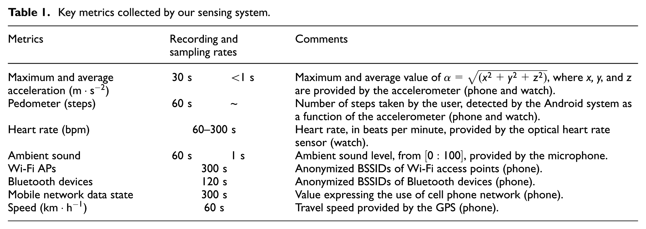
Details of the main metrics collected are listed in Table 1. The “recording” column indicates the frequency at which a metric is saved, while the “sampling” indicates the frequency at which the system acquires raw data from sensors. The average speed of movement of the user’s phone and watch, called the acceleration (or linear acceleration), is recorded every 30 s, along with the maximum speed in order to detect sudden unusual gestures. Note that the linear acceleration is equal to $\sqrt{(x^2+y^2+z^2)}\mathrm{m}·{\mathrm{s}}^{-2}$ , where x, y, and z are the acceleration along each axis of the device, excluding gravity. Other metrics collected by the phone include contextual data such as microphone readings (level of ambient noise) and network data. Further information about the specifications of this system can be found in Faye et al. ⁷

Table 1.

Key metrics collected by our sensing system.

Metrics	Recording and sampling rates		Comments
Maximum and average acceleration ( $\mathrm{m}·{\mathrm{s}}^{-2}$ )	30 s	<1 s	Maximum and average value of $\alpha =\sqrt{(x^2+y^2+z^2)}$ , where x, y, and z are provided by the accelerometer (phone and watch).
Pedometer (steps)	60 s	~	Number of steps taken by the user, detected by the Android system as a function of the accelerometer (phone and watch).
Heart rate (bpm)	60–300 s		Heart rate, in beats per minute, provided by the optical heart rate sensor (watch).
Ambient sound	60 s	1 s	Ambient sound level, from $[0:100]$ , provided by the microphone.
Wi-Fi APs	300 s		Anonymized BSSIDs of Wi-Fi access points (phone).
Bluetooth devices	120 s		Anonymized BSSIDs of Bluetooth devices (phone).
Mobile network data state	300 s		Value expressing the use of cell phone network (phone).
Speed ( $\mathrm{km}·{\mathrm{h}}^{-1}$ )	60 s		Travel speed provided by the GPS (phone).

Data collection

The platform detailed above allowed us to collect data, using a smartphone (LG Nexus 5) and a smartwatch (Samsung Galaxy Gear Live), both running Android 5.1.1. Data were collected from 13 participants working at the University of Luxembourg in the same building and over 13 different days. Each participant was systematically subjected to the same requirements: (1) wear the devices for 1 day, from 10:00 to 23:59, (2) complete an activity diary, and (3) sign an informed consent form to accept the privacy policy of the study.

Figure 1 shows the geographical distribution of our dataset over the 13 participants. These traces are largely concentrated in one area—the participant’s workplace. In most cases, the remaining traces represent commuting activities or meetings in specific places.

Figure 1.

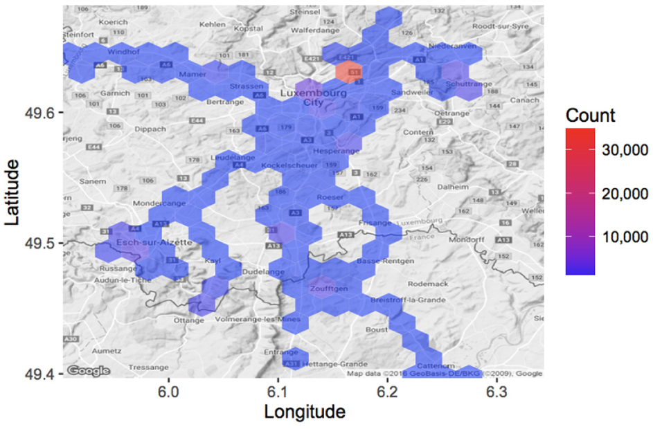
Geographical distribution of our dataset.

Figure 2 shows the hourly breakdown of two types of mobility over our dataset. The red bars represent physical activities, while the blue bars represent activities where the user is in a motorized vehicle. Physical and vehicular activities have been determined using the Android activity recognition application programming interface (API) integrated in our sensing system, and they have been validated using the activity diaries. Overall, we see a fair distribution of physical activities, except in the afternoon, when, for the most part, participants are sitting in their office. Vehicular activities occur predominantly in the evening, when participants return home or take part in some form of social activity. Physical activity also appears to peak around 20:00 when some users participate in a sport.

Figure 2.

Mobility distribution of our dataset.

Energy saving strategy

The provision of a sensing system launched as a background service represents a potential burden on the batteries of the devices used, which are not renowned for their longevity. As described in Faye et al., ⁷ it is therefore critical that we make every effort to save energy. By optimizing data transmission, recording frequency, and the devices themselves (e.g. optimizing default running services), we find an autonomy gain of about 287% for the smartwatch (13.5 h vs 4.7 h with high transmission, harvesting, and recording frequencies) and on the order of 189% for the smartphone (15.7 h vs 8.3 h). Figure 3 represents the energy-expenditure profile of the equipment used. The blue and the orange areas show measurement points for both device—blue for smartphones and orange for smartwatches. The trend line in the middle of each area is a local regression line representing the tendency of these recordings. Overall, we see that our system can easily work for at least 12 h, despite all the sensors being used in conjunction with the low energy capability of the smartwatch. For its part, the smartphone obviously has better capabilities, which are, however, used quite heavily due to its role as a relay point between the watch and the Internet. These energy profiles give us good reason to believe that our system will function for longer periods of time on newer hardware with better batteries. Recent studies performed at SnT, University of Luxembourg, have shown that such a similar sensing system can work for more than 20 h, whatever on a smartwatch (LG Watch Urbane 2) or a smartphone (LG Nexus 5X).

Figure 3.

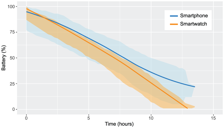
Energy-expenditure profile of the smart devices.

Exploring sensor categories

Understanding human activity and mobility patterns is a fundamental prerequisite in providing context-aware mobility services. Traditionally, characterizing human mobility has depended solely on data available from cellular networks and Global Positioning System (GPS) devices attached to the subject whose movement or activity pattern is under study. However, the proliferation of smart devices equipped with a rich set of high-precision sensors has caused a paradigm shift in the provisioning of mobility- and activity recognition–based services. Activity recognition applications make use of these sensors to detect the physical activities the user performs such as standing idle, walking, running, or driving a car or bicycle. Several studies have been conducted in these emerging research fields; interested readers can refer to existing surveys.^8,9

In this section, we describe three popular categories of sensors in order to provide the reader with a broad view of the relationship between mobility and sensing systems. Relying on our dataset, we discuss and propose for each category original ways of analyzing user mobility. The conclusions of this section will serve as the basis for the generation of a daily mobility profile in the next section.

Motion sensor metrics

According to the literature, ³ motion sensors are among the most used both in specific research connected with movement detection and more general studies focused on user travel patterns. These sensors, typically three-axis accelerometers, can accurately trace the movements made by a device. For example, in Castignani et al., ¹⁰ the authors investigate how motion sensors can be used to detect risky driving events and develop a platform for monitoring driving habits. In addition to these sensors, GPS subsystems fall into this category, because apart from allowing positioning of an object or user in space at a larger scale, they provide comprehensive travel data (e.g. speed). The GPS sensor is the primary positioning sensor on smartphones. It determines a device’s physical location by returning its longitude and latitude coordinates.

Figure 4(a) provides a fundamental diagram that identifies three main categories of mobility: still, physical, and in-vehicle activities. At a specific time, each point of the graph conflates three values measured by the smartphone: maximum linear acceleration, average linear acceleration, and GPS speed. The set of points is extracted from our dataset, without distinction between users. Each point is displayed in a different color corresponding to the activity the user was performing based on data recorded at the time, validated using the activity diaries. We can see a clear trend between three types of activity. First of all, trips made by cars or in motorized vehicles (green) seem clearly independent of linear acceleration, but are closely correlated with GPS speed changes. Conversely, activities causing bodily energy expenditure further stimulate the accelerometer, to a relatively low extent when walking, becoming much stronger when running. Between the two, inactivity (blue) logically causes little response over the axes.

Figure 4.

Fundamental activity diagrams: (a) smartphone and (b) smartwatch.

Consider the case of two users with similar profiles in our dataset: P1 and P11. Each uses their own car for commuting. The coefficient of variation of the speed given by GPS is 1.27 for P1, against 0.7 for P11. This indicates a more constant speed for P11, unlike P1, for whom variations in speed are more frequent (due to congestion, for example). Regarding maximum linear acceleration, it is 0.63 for P1, against 0.71 for P11, suggesting similar driving behavior.

This explains how we can easily distinguish several classes of fundamental activities. Figure 4(b) gives us a similar graph created with data from the smartwatch. As users wear smartwatches on their wrists while traveling, we can clearly see more information about sudden movements, especially those made in a vehicle.

Physiological metrics

Physiological sensors can be used to capture electronic signals from the human body. Such a signal may be electrocardiographic (ECG) data which can be used to infer a user’s stress and emotion level.^11,12 This type of data can serve as an indicator for capturing driving stress experienced by users. When users are considered collectively or as groups, this information has the potential to identify critical geographical or temporal points, that is, places that are perceived as dangerous or perceived negatively by the majority of users, as depicted in Figure 5. With this information, it would be possible to supply a mobility monitoring system that encourages individual users or a group of users to drive on roads that avoid places they usually perceive negatively.

Figure 5.

Stress zones in our dataset.

In terms of recording on a device, it is quite difficult to compare different absolute physiological data, because these can vary greatly from user to user. However, it is easy to imagine a system that measures relative data, such as a coefficient of variation, at regular time intervals.

In the reminder of this article, we do not consider this type of data. While physiological data seem useful for understanding stress and other feelings experienced by the user, it is too dependent on the hardware (smartwatch), consumes energy, and lacks the precision needed to provide a reliable long-term solution.

Environmental sensors

General case

The last category of sensors that can be used to understand human mobility are environmental sensors. Rather than measuring the actions and reactions of users, environmental sensors monitor a user’s surroundings. This category integrates sensors that measure and monitor environmental conditions such as ambient temperature, atmospheric pressure, and illumination. Such sensors include thermometers, barometers, and light sensors.

Several other studies have been based on the use of sensors such as microphones ¹³ and cameras ¹⁴ as a means of automatically recognizing particular places, or simply for identifying the context that users find themselves in. However, the disadvantage of these sensors is that they are too expensive to use effectively. Analysis of audio traces requires microphones to record continuously or at least for a considerable length of time, raising privacy issues. Recording of videos is also expensive—especially on mobile platforms where energy is limited.

In this section, we propose the analysis of network traces, focusing on Wi-Fi traces and their potential for analyzing human mobility.

The case of network metrics

It is worth noting that Wi-Fi and Bluetooth technologies can also be used as environmental metrics to study mobility patterns ¹⁵ and locale characteristics. ¹⁶

Figure 6 shows one of the ways that network traces allow us to understand the movements and interactions a person makes. These figures represent the evolution, over the course of 1 day, of interactions between Wi-Fi access points (APs) and between Bluetooth devices, using a unique numerical identifier generated from their BSSID (Y axis). Figure 6 illustrates the case of two users: P1, who does not move much when at his workplace, and P12, who moves much more, mainly between different meeting rooms and campuses. Both users drive a car. The gray areas indicate when participants are commuting. We can see that both users tend to encounter a large number of Wi-Fi APs, indicating the spatial movements of these users throughout the day. For example, for the first part of his day, user P1 remains in a certain place before moving to another place around 12:00, staying there for an hour, and then returning to the original place. User P12 appears to have much greater mobility, visiting many more places and staying there for less time. It is interesting to see that when P12 goes home around 18:00, he or she continuously encounters multiple Wi-Fi networks, indicating that he or she is moving slowly. Conversely, P1 moves faster and comes across only a few networks. Finally, both participants end their day in a place where the Wi-Fi IDs are unknown: at home.

Figure 6.

Network traces represented as a temporal figure: (a) P1 and (b) P12.

Bluetooth information, although less prolific, seems to provide us with additional guidance on devices in the vicinity. However, the scale is probably too low for us to draw any real conclusions using this technology, although some of P1’s traces seem to indicate that he or she travels by public transport (moving at 18:00 surrounded by multiple devices—suggesting he or she may be traveling on a crowded bus or train).

Sensor fusion

To illustrate the possible correlations between certain measurements, Figure 7 shows an example of how we can represent a large number of metrics. With participant P11 as its subject, the figure displays successively (1) activities detected by a native Android algorithm (ActivityRecognitionApi), (2) the user’s heart rate, (3) the linear acceleration of the smartphone and smartwatch, and (4) a variety of anonymized geographical information. This figure allows us to easily understand the different relationships between sensors and visualizes the user’s main activities throughout the day. It is interesting, for instance, to note the relationship between linear acceleration and the detected activities. For example, around 10:00, linear acceleration is detected by the smartwatch alone, suggesting that the user is stationary but moving his arm—probably at his desk. Between 19:02 and 20:12, the user is clearly detected as moving (GPS), but with a low linear acceleration over the two devices. This tends to validate the detected activity, which is being in a motorized vehicle. This is in contrast with the activity between 20:12 and 21:22, where the high linear acceleration suggests that the user is running.

Figure 7.

Example of multiple sensor data representation (P11).

Using graph theory as a way to understand user mobility

To take things further, we wanted to offer a way of representing interactions between users and networks. To do this, we turned to graph theory. Each device or AP that the user scans is shown as a node. Each time the user scans two separate devices or APs at the same time, an edge is created between the two corresponding nodes. The weight of each edge is simply the number of times the user has scanned this edge. The resulting non-directed graph provides quantitative and qualitative information on mobility and user interactions.

The presence of Wi-Fi APs, which are usually stationary, has the potential to identify places, while nearby Bluetooth devices can help to identify the user’s surroundings and have the potential to detect social interaction between device owners.

For example, Figure 8(a) represents user P12’s Bluetooth interaction graph. The color of each node is proportional to its degree. We can see that a large connected component is present, incorporating the devices that the user encountered when at his workplace. We can also see other connected components, each representing a different device or group of devices that he or she met and that never entered into interaction with others. This may well represent an isolated meeting—a person in the street or something similar.

Figure 8.

Wi-Fi and Bluetooth traces represented as a non-directed graph: (a) Bluetooth—P12, (b) Wi-Fi—P1, and (c) Wi-Fi—P12.

A further example directly connected with user mobility is the use of Wi-Fi networks to achieve this type of graph. Using the principles described above, Figure 8(b) and (c) represents the Wi-Fi interaction graphs of P1 and P12. We can clearly see different features. First, P1 has very distinct connected components, including a large matching with his workplace, which has many APs. A connected component models a group of nodes that are connected together, but disconnected from the rest of the network. P12 also has large groups of nodes; however, in this case, there are clear links between each one, indicating slow movement between these groups of nodes or locations. Refocusing on graph theory, we can explore different traditional metrics to characterize mobility differences between these two users. Table 2 gives us an example of some of these metrics. The number of connected components gives an indication of the number of places visited. The “diameter” gives an indication of the size of the largest connected component and on average over all connected components, which can indicate whether or not the user is physically active inside visited places. The average degree does not give us much information. However, the average weighted degree indicates how much time the user spent in each place visited, because it considers the number of times the networks were scanned.

Table 2.

Graph statistics (Wi-Fi).

	P1	P12
Connected components	9	7
Average diameter	1.4	1.6
Maximum connected component diameter	2	6
Average degree	45.8	42.5
Average weighted degree	403.3	109

Extracting mobility profiles and preferences

As we have seen, several metrics can be taken into consideration, and the relationships between them can be used to compute aggregated values such as activities or locations. In this section, we use the conclusions arrived in section “Exploring sensor categories” in order to see how it is possible to create a representative and visual daily mobility profile for a user.

Methodology

With knowledge of the different categories of sensors that are easily and cheaply accessible, we can already make a number of choices. First, as detailed in section “Motion sensor metrics,” the smartwatch is a good candidate for tracing user’s movements and physical activities. However, it is not the most promising solution, because not everyone has a smartwatch. For this reason, as a first step, it is desirable to provide a modular solution, which will, by default, include metrics provided exclusively by the smartphone. Then, as outlined in section “Environmental sensors,” environmental data collected by microphones or cameras would be a good solution if it was better adapted to the equipment we are using (i.e. if it consumed less power and disk space). Network metrics are, however, more appropriate, in particular, those provided by the combination of Wi-Fi traces and graph theory. Finally, we must use anonymized metrics to avoid compromising the privacy of the user. Note that in a real-world scenario, the smartphone can be used as a default device to compute those metrics, while smartwatches can be used as supplementary devices to improve classification accuracy.

Taking these choices into account, we want to create a simple mobility profile, representative of different types of mobility and which is not trivial (i.e. the user cannot provide all or part of it by answering a few questions, such as his favorite means of transport). The graph theory aspects studied above seem to be ideal candidates for this because they are easy to retrieve, inexpensive to obtain in terms of energy (i.e. recording frequency does not need to be high), and they are easily generalizable to several time scales (e.g. hour, day, and week). Thus, the profile we generate uses only a smartphone, recording two groups of metrics constantly and at equal intervals: (1) anonymized (i.e. hashed) Wi-Fi AP BSSIDs encountered by the smartphone, in order to build for each user a graph G similar to the one presented in section “Environmental sensors” and (2) activities performed by the user, only as labels (i.e. post-computed data), with a counter registering the number of times the user performed each activity. Finally, a relationship is created between those two groups by associating a Boolean with each node to indicate whether or not the user was mostly moving (either physically or through some form of transportation). The concrete implementation of the application is detailed in Faye et al. ¹⁷

Mobility metrics

This profile is built on top of four aspects that we consider essential when profiling human mobility.

Number of visited locations

We extract this metric from the sub-graph $G_{\mathrm{still}}$ , which is composed only of nodes where the user was not in motion. To represent this metric, we suggest using the number of connected components of $G_{\mathrm{still}}$ .

In our case, a connected component represents a group of Wi-Fi APs that were scanned at the same location while the user was not in motion, or at a distance that varies depending on the communication range of these APs. These groups are therefore ideal candidates to represent the different places visited by the user.

In order to validate this metric, we sought to compare the values obtained for each user with the number of places calculated using GPS data directly. For this purpose, for each user and for all of their GPS points, we considered a visited place to be a cluster of GPS positions that are not separated by more than a certain distance. Other methods exist, but we have been aiming at achieving the simplest. As depicted in Figure 9, we tested several distances. The best one is around 800 m, where we found a Pearson’s correlation coefficient of 0.93, which confirms the adequacy and accuracy of this value.

Figure 9.

Correlation coefficients vs distance.

Pearson’s correlation coefficient is a classical statistical measure of the strength of a linear relationship between two variables, giving a value between −1 and 1. Spearman’s rank correlation coefficient is a complementary measure, indicating whether the relationship between two variables can be described using a monotonic function.

Urban index

The second aspect we want to consider is the paths between these different places. For this, we consider the complement graph of $G_{\mathrm{still}}$ , namely, $G_{\mathrm{mobility}}$ , which only consists of nodes with moving activities. Based on this graph, we extract what we call an urban index, representing whether the environment in which the user is moving is an urban area.

In order to find the best possible representation, we chose to compare several metrics extracted from graph $G_{\mathrm{mobility}}$ to “ground truth” reference metrics. These reference metrics are generated from two scenarios that consider GPS traces and OpenStreetMap (OSM) data as a basis for representing an urban environment and its importance. The first scenario considers a GPS point to be in an urban environment according to its proximity to residential roads (http://wiki.openstreetmap.org/wiki/Key:highway). The second scenario considers the number of buildings (http://wiki.openstreetmap.org/wiki/Key:building). Using different radius parameters (from 0 to 2000 m), we arrived at the following conclusions:

1. As stated in Faye and Engel, ¹ our first results indicated that the number of nodes present in graph $G_{\mathrm{mobility}}$ is related to the number of residential roads within an ideal radius of 420 m. The more a user moves around in an urban environment, the more he or she will tend to come across Wi-Fi APs. In this case, we find a Pearson’s correlation coefficient (linear) of 0.74. In our current application, we consider this metric to be representative of our urban index.

2. By taking the analysis further and considering the second scenario (i.e. the presence of buildings), our last results at the time of writing this article show a Spearman’s correlation coefficient (i.e. nonlinear) of 0.83. The ideal distance used to acquire the number of buildings is 120 m. These results are obtained by using as a metric the average diameter of the connected components in graph $G_{\mathrm{mobility}}$ . Indeed, the wider the diameter, the greater the density of APs crossed by a user at a given time.

It should be noted, however, that based on the data we have, it is difficult to quantify and qualify what an urban environment is and how important it is. For example, the number of residential roads around a particular location can be as important in a village as in a large city. In the same way, two similar buildings may contain a completely different number of Wi-Fi APs. However, our first experiments tend to conclude that our index is representative and valid.

Spatial exploration

Looking at the complete graph G (i.e. $G_{\mathrm{still}}+G_{\mathrm{mobility}}$ ), we compute an index showing whether or not the user has a tendency to move inside the most important place he or she visited. This metric has a relationship with the number of articulation points of the maximum connected component. The maximum connected component is the connected component that contains the largest number of nodes, while an articulation point is a node whose removal disconnects the component it belongs to, increasing the number of connected components.

In order to validate this index, we compute the average duration of the walks of each user when he or she is at his workplace (i.e. the maximum component). The longer the user moves in a place, the more he or she will tend to “explore” this place. Comparing these values to our index, we found a correlation coefficient of 0.76, which also confirms, to a certain extent, the validity of this index.

Activities

Finally, separate from the graph theory principles, we compute two indexes for each mobility activity: physical activity and in-vehicle activity. These scores simply reflect the proportion of time the user was performing a physical activity or was in a vehicle. They are simply computed by dividing the count of each activity over the total count of all activities. The accuracy is high and was verified using the activity diaries provided by the users and the timestamped data. Indeed, the veracity of the Android activity recognition API has been largely verified by the literature and supported by previous studies. ⁷

Use-case

Figure 10 shows four examples of profiles in the form of a radar chart (or Kiviat diagram, as described in Chang et al. ¹⁸ ) based on data collected on four participants having different characteristics in our dataset. The minimum and maximum axes for each characteristic are determined according to our dataset.

Figure 10.

Mobility profile of P1 (yellow), P7 (red), P11 (blue), and P12 (green).

Participants P1 (yellow), P11 (blue), and P12 (green) drive a car and live in cities which are far from their work, while participant P7 (red) lives near to his workplace and gets around by bike and by public transport, as reflected by his high urban index (i.e. a large number of Wi-Fi APs scanned when moving).

Moving slowly (bus and on foot) allows more APs to be scanned, in comparison with other means of transport, which creates the greatest number of connected components, as reflected in the visited locations.

As introduced in section “Environmental sensors,” participant P12 has a sporty profile, as reflected by his high physical activity score. Conversely, participant P1 does not move much when at his workplace, as reflected by his relatively low spatial exploration index. Note, however, that the spatial exploration index tends to be close for each participant as they share the same place during most of the day on which they participated in the data collection.

Finally, Note that participant P1 is an intermediate case, having results situated in the middle of our experiments. Participant P11 travels more than other participants, as reflected by his vehicular activity score.

Development and evaluation of a mobility assistant

Under the hood: building an android application

Our Mobility Assistant consists of a two-tier client and server application implemented on Android and based on the architecture proposed in Faye et al. ¹⁷ Specifically, the system architecture includes the following: (1) a client-side data recording and processing component and (2) a backend server onto which we offload heavy-duty graph metric computations. The client application records user activity and anonymized Wi-Fi traces to generate a user’s activity profile and intermediate mobility data. Next, the client transfers this data to the remote server through a secure connection. The server then computes and extracts the mobility metrics and sends the result back to the client to be displayed on the user interface. Three main tabs are displayed in the application, namely, Activity, Mobility, and Survey Tabs as described below.

Activity

This part of the application makes use of smartphone sensors and the Android Activity Recognition API to detect physical (walking, running, and on foot), vehicular (in vehicle or on Bicycle), and still (inactive or immobile) activities of the user. These metrics are displayed in a radar chart as shown in Figure 11(a) and serve as input to the mobility feature extraction algorithm. This tab also displays in real time a pedometer reading the number of steps the user has walked since the device was last turned on. Users can also view historical data on step counts and walked distance for the previous 7 days. The range seek bar beneath the radar chart gives the user the flexibility to navigate through his historical activity data.

Mobility profile

This tab, as depicted in Figure 11(b), shows user’s mobility indexes represented in the form of a radar chart. By default, after every 24 h, the client application requests the computation of the mobility metrics by uploading anonymized user activity and Wi-Fi traces to the server.

Contextual survey

In order to label the dataset, we conducted a contextual survey so as to collect real-world mobility information of users, including when, where, and how they move. The survey results are presented in vertical bar charts as depicted in Figure 11(c). By default, the application will prompt the user from time to time, by means of notifications, to complete a survey questionnaire regarding his or her mobility activities. Users can change this configuration in the settings tab. However, to avoid overwhelming the user with notifications, a notification is only sent once as long as the user’s activity remains unchanged.

Figure 11.

MAMBA mobility assistant: (a) activity tab, (b) mobility profile tab, (c) contextual survey tab, and (d) MAMBA open trip planner.

Finally, as described below, the mobility assistant also has a section dedicated to a trip planning application based on the open-source software OpenTripPlanner (OTP; http://www.opentripplanner.org/).

Use-case: multimodal trip planning

One of the key objectives of this application is to use the obtained results as input to a context-aware multimodal trip planning software. This software is currently being developed as part of a national funded project, MAMBA. In particular, our trip planner is built on top of OTP.

OTP is an open-source multimodal trip planner. It bases itself on OSM and General Transit Feed Specification (GTFS) data to build a graph of transit networks. OSM provides the streets’ data, whereas the GTFS supplies the location of transit stops and the timings of the vehicles that visit those stops. OTP creates travel time contour visualizations by computing the shortest path between a source and a destination under a given set of constraints.

Ideally, when planning a trip with OTP, the user provides the source and destination addresses to the application which in turn displays the available trips’ information to the user. The MAMBA mobility profiler, thanks to our mobility profiling algorithm, seeks to anticipate this scenario by automatically considering the user preferences (e.g. mode of transportation and type of roads to consider) and give him or her real-time transportation advice. For example, based on the user’s activity, mobility behavior, and other external data sources, the application can notify him or her about when to leave home for work or for a meeting. The application could also inform the user about his or her estimated time of arrival, advises him or her not take his or her personal car to work but rather to take a public transport due to unavailability of parking space, perhaps because of an event at/near his workplace. A screenshot of the trip planner is shown in Figure 11(d).

In order to evaluate our application, a first data collection campaign has been performed. Further results and discussions, which are out of the context of this article, will be given in a future publication.

Additional metrics: the case of Bluetooth

Bluetooth has been used in the past by others^19–21 for characterizing different human behaviors to identify among other things the mobility and environment of users. In addition to the findings presented in this article, we discuss below the potential of combining the use of Bluetooth to our system.

Bluetooth’s application-centric nature, compared to Wi-Fi’s network-centric nature, has the potential to further improve a sensing system by profiling not only the user’s surroundings by also detecting activities and social interactions.

Using Bluetooth traces would allow to characterize different information about the environment. Moreover, it is clear how the potential of this technology, when used to its fullest, can further improve our profiling methodology.

By analyzing Bluetooth’s discovery characteristics, we can add more information to our network traces. By observing manufacturer- and class-specific data within discovery packets, we can enhance our fingerprinting. Analyzing such data will help us to identify and classify nearby devices by observing their class type (e.g. smartwatch, smartphone, car, or TV).

Furthermore, it is important to differentiate between standard Bluetooth and Classic Bluetooth (BC or Bluetooth Smart). The BC implementation, introduced from the protocol specification 4.0, is not backwards compatible with standard Bluetooth as it uses different physical and link layers. This particular version has gained its popularity due to its low energy requirements and its very advantageous range (i.e. up to 100 m in its current version 4.2).

In previous work, we tested the feasibility of classifying a vehicular environment by contextualizing our surrounding through Bluetooth discovery data. ²² By looking at the type of discovered devices while driving, we observed how different device types are correlated to specific road types (e.g. TVs will only be discovered in urban areas). In a similar way by analyzing the amount of devices discovered over time, we can deduce a probable traffic situation (e.g. congested if many vehicles are discovered in a specific context).

Knowledge about the environment and traffic conditions could directly offer added value to improve our mobility profiler. As an example, Bluetooth could help complement Wi-Fi in our urban index (section “Urban index”). Furthermore, for Bluetooth-only discovered devices, we could extend this concept to a different mobility index capable of identifying, based on name and type of a device, the probability of it being either fixed (e.g. TV, iBeacon) or mobile (e.g. car, smartphone).

Very recently (December 2016; https://www.bluetooth.com/news/pressreleases/2016/12/07/bluetooth-5-now-available), the Bluetooth special interest group finally launched the latest version of this technology. Bluetooth 5 promises up to four times the range of version 4.2 and up to eight times the amount of data (https://www.bluetooth.com/specifications/bluetooth-core-specification/bluetooth5). These figures, together with the promise of an even better coexistence with Wi-Fi, are promising for whether this technology will be adopted massively in the coming years. In our particular case, the extended range could allow us to identify even further devices and thus improving the overall accuracy of the profiler.

In conclusion, Bluetooth in its current and future different forms and implementations can and should be used for a multitude of human mobility-related applications.

Conclusion

In this article, we have explored different ways of studying user mobility, proposing creative ways in which the study can be achieved. We used an open-source platform and an anonymous dataset collected over 13 participants. In particular, we used network and activity data acquired from smartphones and smartwatches. In addition to study the interest of using physiological and motion data, we show that the use of network data has a good potential for describing and characterizing a user’s mobility. In particular, combining graph theory, activity data and Wi-Fi traces allow to characterize specific aspects of a user’s mobility behavior, such as his or her physical activity and number of visited locations. Using these findings has allowed us to propose a way of describing user mobility by creating a profile in the form of a radar graph. This profile offers a simple and inexpensive way to analyze five characteristics showing user preferences and mobility choices.

Even if the metrics presented in this article remain very general, we really think that theories allowing the representation and abstraction of large datasets, such as graph theory, can bring a greater level of detail to human mobility characteristics.

The work presented in this article is empirical, in the sense that it details a set of ideas based on a multimodal dataset and several scenarios. One future work, which has already been carried out through a few publications,^6,7 is to go deeper into each of the aspects mentioned in the article.

In future work, we intend to take advantage of these conclusions, which provide clear inputs to support intelligent mobility systems such as navigation services as described in section “Development and evaluation of a mobility assistant.” It is easy to imagine this kind of service, taking into account different types of profiles (e.g. automatic selection of mode of transportation, favorite route, and places). While the profile generation method suggested in this article remains an illustrative example of the potential for sensor systems, we also plan to formally validate the relationship between graph theory and mobility patterns, in addition to introduce new topologies and graph theory aspects, such as dynamic graphs and time-dependent components.