
Abstract
Clustering techniques in wireless sensor networks have been widely utilized for their good performance in reducing energy dissipation and prolonging network lifetime. Once the cluster heads have been decided, the allocation of member nodes in the cross coverages formed by two or more clusters is critical to keep an energy balance on the cluster heads. In earlier studies, however, the allocation of member nodes simply depends on the distance or degree (the node number within the cluster heads’ communication radius) and, therefore, could cause imbalance to the cluster heads’ load and further degrade the whole wireless sensor network. To maintain the load balance of the cluster heads, in this article, game theory is introduced into the allocation problem of the member nodes. Before using the game theory approach, the number and distribution of cluster heads are first checked. If the cover rate of the cluster heads is low, then the node(s) uncovered by any cluster are randomly selected as new cluster head(s) to attain the cover rate required in the article. Furthermore, the number of cluster heads in a monitoring region is restricted. Finally, a game-based, energy-balance method is proposed and applied in the cluster-based routing protocols to improve their performance. For verification, the proposed method is embedded into the localized game theoretical clustering algorithm and hybrid, game theory–based and distributed clustering algorithm, which are two game theory and typical cluster-based routing protocols. The experimental results show that both of the improved protocols do balance the loads of the cluster heads and achieve better performance than their original versions in spanning the lifetime and balancing the energy in wireless sensor networks.
Introduction
Wireless sensor networks (WSNs) have attracted broad attention from many research communities in recent years for their good performance. Their rapid development has mainly benefited from the vast advancements in hardware and wireless communication technology. The sensor nodes are basic elements of WSNs, which are characterized by their small volume, cheapness and availability. A large number of sensors can wirelessly communicate with one another. Each node senses local physical data and then forwards it to a remote base station (BS) called a sink. 1 WSNs have already been broadly applied in various fields, such as environmental monitoring, 2 agriculture, health care, 3 disaster management, 4 domestic systems and surveillance systems. 5 However, the networks face a common problem in that a sensor node equipped with battery is difficult to recharge or replace since it could be deployed in untouchable environments. 6 Thus, efficient energy management that prolongs the network lifetime becomes a hot spot.
Usually, the deployment of sensors is random or regular in a monitoring region. For energy saving, they must be efficiently organized. Clustering, an effective organization technique, is used to group the sensor nodes into independent clusters. In clustering, the role of each sensor node is the same as each of the others but can take on different responsibilities. The sensor node that serves as a cluster head (CH) is responsible for collecting data from its member nodes (MNs), aggregating the data and forwarding the aggregated data to the BS. The sensor node that serves as an MN is for sensing data and sending the data to a CH in a direct or indirect way. Cluster-based routing is known as hierarchical routing. The hierarchical routing schemes include the following protocols, such as low-energy adaptive clustering hierarchy (LEACH), 7 hybrid energy-efficient distributed (HEED) clustering, 8 distributed weight-based energy-efficient hierarchical clustering (DWEHC) protocol, two-level hierarchy LEACH (TL-LEACH), 9 base station–controlled dynamic clustering protocol (BCDCP), 10 threshold sensitive sensors energy or efficient sensor network protocol (TEEN). 11 In these protocols, the CHs suffer from the extra workload. As a result, once a normal node with less energy is chosen to be a CH, it will prematurely run out of power. Thus, how to select an appropriate CH is important to balancing the energy consumption in WSNs. In addition to hierarchical routing methods, there is flat routing. The typical flat routing protocols include flooding and gossiping, sensor protocols for information via negotiation (SPIN), 12 directed diffusion (DD) 13 and greedy perimeter stateless routing (GPSR). 14 In flat routing protocols, all of the nodes take on same tasks and functions over the whole network, and the data that the sensors obtain are sent hop-by-hop by flooding. However, in comparison with hierarchical routing, the protocols based on flat routing have difficulty in being competent for large-scale networks. Thus, the clustering routing becomes a hot research branch of routing technology in WSNs because of its various advantages, for example, more scalability, data aggregation/fusion, less load, less energy consumption and more robustness.
Game theory (GT) is usually used to study rational individual activities in interest conflicts. 15 In recent years, it is introduced for the optimal selection of CHs in WSNs. It first models all of the sensor nodes; in the game, players are given different interests according to various strategies. After a competition of their interests against one another, a better balance in the energy load will be achieved. 16 In the CHs’ selection game, the CH consumes more energy than the MNs. Thus, each player does not want to become a CH for its own interest. However, each node must provide services for the global interest. In this situation, it is important to devise a GT-based and energy-balance protocol between the minimization of the energy expenditure and the effective provision of necessary services. 6 clustered routing for selfish sensors (CROSS) 17 is the first protocol to use the GT to find the optimal CHs in the clustering routing. In CROSS, each sensor node is a player in the game. The strategies are devised under different payoffs that motivate players to compete for their own interests. Finally, the decision of a player (node) to be a CH or not relies on the equilibrium probability derived from the GT-based method. However, since the nodes’ transmission capability is not restricted, CROSS is not suitable for practical applications. To meet the requirements in real networks, a localized game theoretical clustering algorithm (LGCA) 18 is presented. Each player communicates only with its neighbours within a fixed communication radius. Thus, LGCA is more suitable for real scenarios than CROSS. To further improve the performance of LGCA, a hybrid, game theory–based and distributed clustering algorithm (HGTD) 19 is proposed, and it offers some fined-grained payoff definitions for each node under different strategies in local games and achieves higher performance over the lifetime of networks. LGCA and HGTD use the same GT strategies as CROSS. The main difference between LGCA and CROSS is in the communication ability: LGCA is restricted, while CROSS is not. In addition to the fact that the communication ability of each node is restricted, HGTD gives concrete definitions of the payoffs under different strategies and uses an iteration procedure to remove the neighbouring CHs within their proximity. In this article, we mainly use GT to analyse the optimal allocation of MNs in cross coverages by two or more clusters after the election of the CHs. In addition, in the CH-selection phase, the number and the distribution of the CHs are also considered to be important factors that affect the network performance. The main contributions of this article are listed as follows:
We first deduce an optimal number of CHs. If the distribution of CHs is uneven and their number is less than the optimal number, then new CH(s) will be automatically selected on the basis of a preset threshold.
We apply GT to determine the allocation of the sensor nodes in the cross coverage by two or more clusters. Their appropriate allocation makes the CHs and the whole network have better energy balance.
We give payoff definitions that are related to the energy consumption for the CHs in cross coverages. In the game, we also consider two distances: one distance is the distance between the CHs and normal nodes and the other is the distance between the CHs and the BS. All of the considerations are devoted to constructing an energy-efficient network.
Related work and motivation
In the cluster formation phase, it is important to appropriately allocate nodes in cross coverages to different CHs to balance the energy consumption. In earlier papers, there are two simple but typical allocation schemes7,18,19 that are used to address the issue. One is the distance scheme in which MNs join the nearest CH to form clusters; the other is the degree scheme in which MNs join the CHs with the smallest degree. LEACH 7 does use the distance criterion. For each non–cluster head node, joining a cluster or not depends on its received signal strength of CHs’ advertisement. When a sensor node receives signals from ambient CHs, it selects and joins the cluster for which the signal received from the CH is stronger than that from the other CHs. In general, the nearer the distance between two sensor nodes, the stronger the received signal. An LGCA has a similar allocation scheme as LEACH. It is unlikely that a HGTD uses the degree criterion in the clustering formation phase. The non-CH nodes will join the CH that has the smallest node degree. To demonstrate the difference between the two schemes, simulations are given here using the parameters shown in Table 1, and the simulation results are given in Figures 1–8, in which six final CHs are considered to reach a good demonstration.
Simulation parameters.


Distance criterion allocating the nodes in the cross coverage.

Six random CHs in LEACH when the monitored area is 1 × 10⁴ m2.

Number of member nodes of each cluster in LEACH.

Energy expenditure of each CH in LEACH.

Degree criterion allocated the nodes in the cross coverage.

Six selected final CHs in HGTD when the monitored area is 1 × 10⁴ m2.

Number of member nodes in each cluster in HGTD.

Energy expenditure of each node in HGTD.
In Figure 1, the two large red and green dots denote the CH in the left region and that in the right, respectively. Normal nodes are represented by small red or green dots in the cross coverage formed by two clusters and will join the cluster according to the distance criterion. Although the left cluster has more normal sensor nodes than the right cluster, the nodes in the cross coverage select the closer CH to join. Thus, it must cause the CH in the left cluster to expend more energy than that in the right cluster.
LEACH is used to show the results based on the distance criterion. In Figure 2, the CHs are randomly selected and their distribution is uneven in the monitored region. Figure 3 clearly shows that the distance criterion causes Clusters #1 and #5 to have more MNs than the other clusters. Correspondingly, CHs 1 and 5 consume more energy than the others in Figure 4.
In Figure 5, the large red and green dots also denote the left and right CHs, respectively. Normal nodes in the cross coverage formed by the two clusters will choose to join a cluster according to the degree criterion. Although the cluster in the left has more normal sensor nodes than that in the right, the nodes in the jointly managed zone will choose to join the CH that has fewer nodes. Since the green CH will serve the far nodes to raise its degree, the result is that the green CH will expend more energy than the left CH.
In Figure 6, the HGTD protocol is used to show the results for the degree criterion. It is clear that the distribution of the CHs is relatively even. However, the degree criterion in HGTD causes Clusters #1, #2 and #6 to manage more MNs than the other clusters, which is shown in Figure 7. It can also be seen that CHs 1, 2 and 5 spend more energy than the other CHs in Figure 8.
From Figures 4 and 8, it is obvious that the nodes’ allocation in the cross coverages will seriously influence the CHs’ energy balance.
From the above simulation, we found that both of the allocation criteria have their own weaknesses. Motivated by GT, in this article, it is used to allocate the MNs in the cross coverages to different CHs. Next, we plan to use GT6,20 to model and address the situation. Additionally, before the nodes’ allocation in the cross coverages, the number and the distribution of the CHs are first considered for the purpose of achieving higher performance of the WSNs.
Overview of the system model
Network model
The proposed method is mainly applied in the two-layer network model–based protocols, which are based on the two-layer network model. 21 In the model, the sensors in the bottom layer are responsible for collecting the data and then forwarding the data to the corresponding CH in the top layer. Finally, the CHs aggregate the data and send the data to a BS. In these protocols, the following assumptions are required:
Each node is equipped with a unique ID, which is used to label the data source;
Once the sensor nodes are placed in the monitoring region, their positions never change;
The battery energy of all of the nodes is the same and cannot be recharged, while the energy of the BS is not limited;
The distance can be measured according to the wireless radio signal power;
Each node can adapt to its transmission power according to its distance to the destination.
The radio model
A two-layer radio model 6 is shown in Figure 9.

Two-layer radio model.
To compute the nodes’ energy consumption in the model, the cost of a k-bit packet transmitted to the destination is calculated by equation (1) in Jin et al., 22 Heinzelma et al., 23 Shokouhifar and Jalali 24 and Sabet and Naji 25
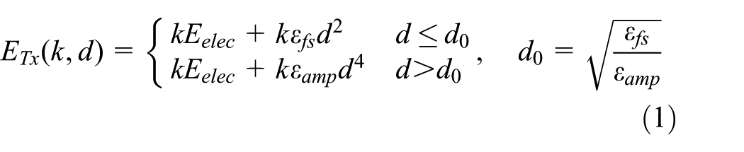
where

where
Proposed method
In this article, first, the optimal number of CHs is deduced for the monitoring region. Then, the distribution of CHs is checked, and if the number of the nodes that are uncovered by all clusters exceeds a given threshold, then we will randomly select new CH(s) among the uncovered nodes to meet the node coverage rate in a finite number of iteration steps. Next, the GT is introduced to model the allocation of the nodes that exist in the cross coverages.
Restriction on the number of CHs
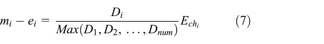
Through a number of observations, we found that the number of CHs in a certain region is vital to the proposed method. If the CHs are beyond a certain number, then they will consume more energy for their remote communication with the BS in the WSNs. Additionally, we first give the following formula19,21 to compute the former optimal number

where

Many protocols are devoted to selecting CHs to balance the energy and span the lifetime in a WSN. In the CH-selection phase, to avoid having other tentative CH(s) in the communication radius of a tentative CH, in this article, we select only the attained tentative CHs that have no neighbouring tentative CH(s) as the real CHs. We assume that

where
Detecting the tentative CHs’ distribution and finding the same point sets in the cross coverages
In the initialization phase, the ‘Start’ message is broadcasted by the BS, and all of the MNs are assumed to be able to receive the message. According to the received signal strength, each node can calculate its distance to the BS. Then, each node broadcasts a ‘Hello’ message to the nodes within a radius of R. Finally, everyone knows all of their neighbours by receiving the ‘Hello’ messages. Additionally, in this article, our approach starts after the tentative CHs’ selection. We first check the distribution of the tentative CHs and then find the sets of the nodes in the different cross coverages; next, the GT method is used to allocate the sensor nodes to appreciate the clusters.
Algorithm 1 is proposed to check the distribution of the current CHs and to reselect new CH(s) among the uncovered nodes. In this algorithm,


The algorithm below is used to determine the point sets in the cross coverages (Table 2). This procedure consists of four steps. First, the CHs send the message CHID within their specific communication radius; second, normal nodes in the cross coverages receive the message and record it; third, normal nodes send messages that concerned with its node ID NodeID, the number of CHs NumofCH and the CHs’ ID CHIDs in their specific radius; and finally, the normal nodes in the cross coverage exchange messages with one another. Next, each normal node begins to compare the number of CHs, NumofCH, of the node ID NodeID within its radius. If the number for the two nodes is not equal, then it is clear that they are not in the same cross coverage. If the number is equal, then the normal nodes continue to compare their CHIDs. If their CHIDs are the same, then they belong to the same cross coverage. The process is not finished until all of the point sets in the cross coverages are formed.
The payoffs for the simple two-player clustering formation game.
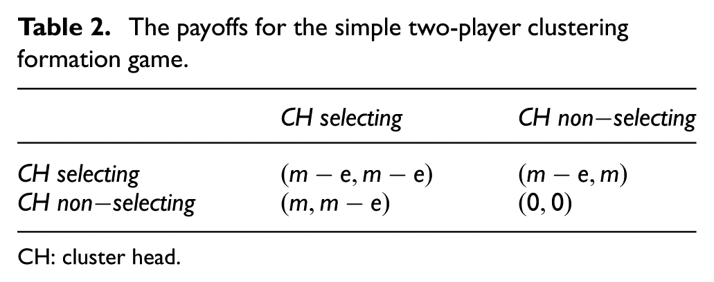
CH: cluster head.
Game application and equilibria analysis
The GT algorithm in this article works in the phase of the clustering formation, which lies in the red region in Figure 10. In Figure 10, first, the data stream is divided into frames, and each frame is also divided into time slots. Each cluster member is allocated one slot. When all of the clusters have been constructed, the first cluster member will be awaked. In the time slot of the MN, its data will be forwarded to its corresponding CH and then the next node repeats the actions similar to the previous node in rapid succession. Additionally, the time slots also contain the data with a guard period if needed for synchronization. Finally, the CHs will aggregate all of the collected data and send it to the BS.

Work flow with new method (red regions).
Next, we model the game. In Figure 11, the big white circles denote the game players (CHs) and the small white circles (MNs) represent the selected objects in the cross coverage simultaneously covered by clusters A, B and C; the players A, B and C compete for each selected node (MN;

Game with three players (CHs) competing for each normal node in the cross coverage.
To allocate the normal nodes in the cross coverage into an appreciated cluster, the clustering competition node game (CCNG) is proposed. The responsibility of a CH in the game is to collect data from the MNs that lie within its radius and to send the aggregated data to a BS, which is usually placed far from all of the sensors. We model the game as
Let us now discuss the possible equilibria in the case of two players. Their payoffs are summarized in Table 2. It is obvious that the game strategies are symmetrical because the payoff is only related to the strategies and has nothing to do with who they are.
Both the strategy
Furthermore, we assume that N players play the game, and we let

in which the payoff is
Proposition 1. For the symmetrical clustering game, the strategy
Proposition 2. For the symmetrical clustering game, the strategy
Proposition 3. For the symmetrical clustering game, the strategy where a single player plays
Proposition 4. For the symmetrical clustering game, no symmetric pure strategies with Nash equilibria exist.
To permit the game in the article to have symmetrical Nash equilibria, we must allow the players to play mixed strategies, which means that the players choose their strategies randomly following a probability distribution. In other words, every player now has a probability of selecting a node in its cross coverage as its member and a probability of not doing so. Let us denote the probability of playing
After the above analysis, we will compute the equilibrium probability
Theorem 1
For the symmetrical clustering game, a symmetric mixed strategies Nash equilibrium exists, and the equilibrium probability p that a player declares itself as a cluster head is

where
Calculating equilibrium probabilities
For CH

where
where
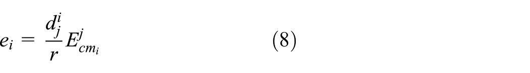
Let
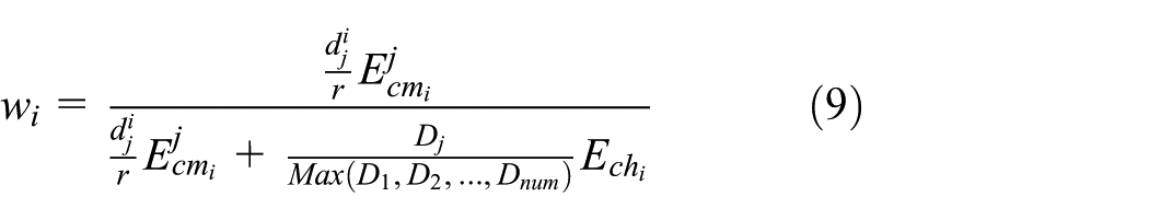
In equation (9), it is clear that

in which
where

in which N denotes the current round number, and
When the ith CH plays the game, its payoff mi is calculated by equation (6). Next, the values

where
where
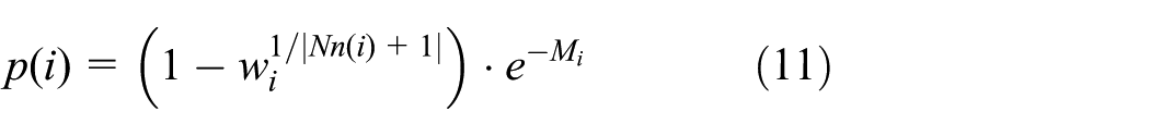
Decision of the normal nodes
When

Then, we obtain in Figure 12,

In equation (15),

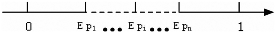
Regular equilibrium probability.
If the value of
The main goal of the proposed algorithm is to balance the energy consumption for all CHs by the allocations of the nodes in the cross coverages at the clustering formation phase. Our approach is not completely independent from the CH election protocols, and any other cluster-based routing protocols can use it to obviously improve their performance.
Performance evaluation
Our method is mainly applied in the setup phase, as given in Figure 10. Additionally, allocating the nodes in the cross coverages and reselecting better CHs are our concrete work. In this section, we attempt to further analyse the time consumption of our method.
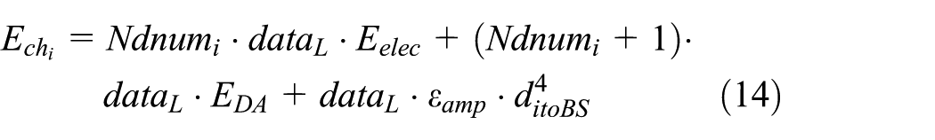
In detail, on the basis of the CH-selection methods, we first restrict the optimal number of CHs; under the restriction of the optimal number of CHs, we randomly select the uncovered nodes with the larger coverage ratio and the more residual energy to be the CHs. Once the optimal number of CHs is more than or equal to the optimal number set by us, the iteration process will terminate and be clear in Algorithm 1. In this process, the
On the basis of the above analysis, it can be seen that the energy consumption is only cost in the information exchange between
in which

Communication among MN, CH and BS.
The above formula can be further divided into two parts: one part is

and the other part is
The first of the above two formulas is the phase in which the distribution of CHs will be checked and new CH(s) will be generated if CHs do not attain the cover ratio set by us. It assumes that

in which
However, the worst case of selecting new CH(s) from

The second formula is the phase in which the BS decides which CHs will manage the nodes in the cross coverages. This approach assumes that the total number of MNs in the cross coverages is

in which
The cover ratio in this article can maintain a higher value than that in earlier papers. Thus, there will be fewer isolated nodes, which can save more time than the other approaches. It is worthwhile to mention that the
Simulation results
In this section, we describe the simulations. The parameters used in the experiments are given in Table 1. Additionally, the simulation results are given in this section. Then, we evaluate the performance of the proposed method by analysing the results.
Simulation environment
A rectangular area with the size

In addition, the predefined parameter

Now, we can evaluate the performance of our approach under the following situations.
For various values of the network size S (L×W m2) of the network, the protocols LGCA and HGTD combined with our approach, which are, respectively, called the improved LGCA and HGTD, are compared with LGCA and HGTD themselves. The communication radius R has already been calculated by equation (17). The values of S are chosen as 50×100, 100×100, 100×150, 150×150, 150×200 and 200×200 m2. The BS is located on position (L/2, W + 50), and the node density
Analysis of results
First, we show the performance in terms of the energy consumption. Figure 14(a) and (b) is the results of LGCA and the improved LGCA, separately, at the 200th round. It is clear that the energy allocation of B is more even than that of A. C and D are the results of HGTD and the improved HGTD. We can see that the CHs in the improved HGTD use their energy evenly but the original HGTD does not. This finding indicates that the GT plays an important role in balancing the energy consumption.
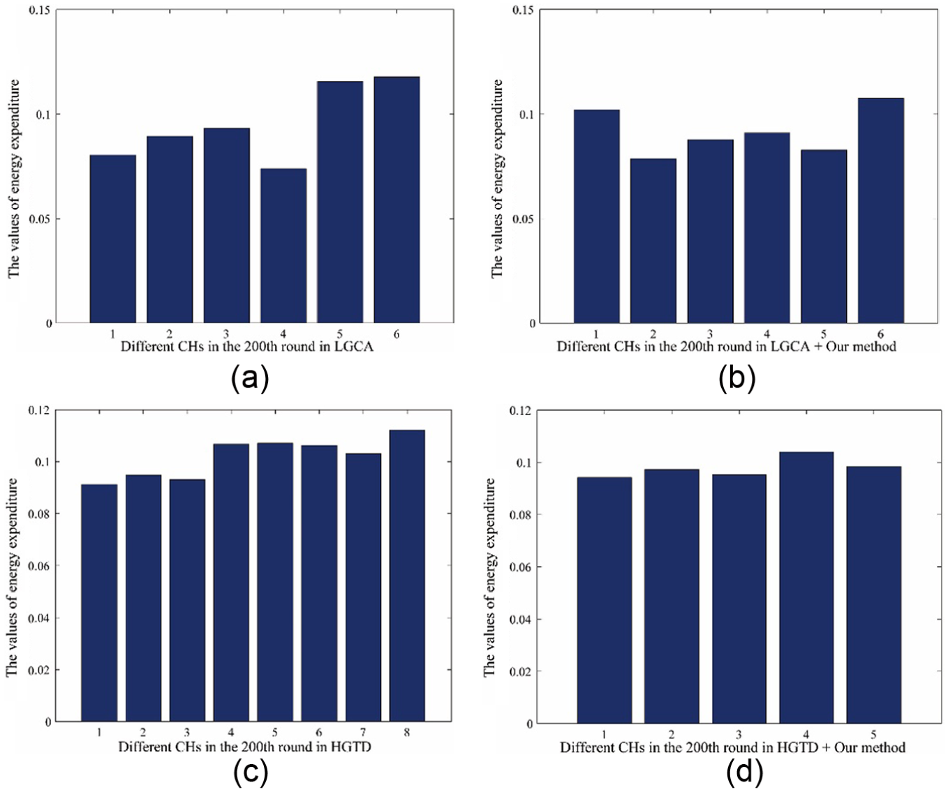
Comparison of the improved protocols with their original versions in terms of the energy consumption at the 200th round when S = 1 × 10⁴ m2: (a) LGCA, (b) improved LGCA, (c) HGTD and (d) improved HGTD.
Figure 15 compares the number of CHs in LGCA, HGTD and their improved versions for S = 1×10⁴ m2. The original optimal number of CHs is derived from equation (3). The number of CHs in the improved protocols is lower than the original optimal number and has a small variance, while LGCA and HGTD show the opposite. It is clear that the variance of the number of CHs is too large to maintain their energy balance.

Original optimal number of CHs in equation (3), and comparison of the optical numbers of the CHs among LGCA, HGTD and their improved versions when S = 1 × 10⁴ m2.
In WSNs, the network lifetime is a very important evaluation criterion for clustering protocols, and it is defined by the lifespan of the first node, which depletes its energy in the network. Figure 16 shows a comparison of the network lifetime among LGCA, HGTD and their improved versions with different network sizes S. In terms of the network lifetime, this figure shows that the improved protocols outperform their original version in all cases of S. With the increase in S, all protocols have a downward trend in S, which means that the CHs cost more energy to send their information to the BS. Additionally, it shows that HGTD is much better than LGCA, which indicates that the CH-selection mechanism is important to the energy balance. The improved protocols have longer lifetimes than their originals. The reason is that our method in the clustering formation phase has good performance. Especially when the monitoring region S is chosen to be 200×200 m2, the improved LGCA outperforms HGTD. The figure also indicates that our method can significantly improve the performance of the original protocols. When the monitoring region S is 100×150 m2, although the improved LGCA is better than the original LGCA, the efficiency is not obvious. The reason is that the selection of CHs in the original LGCA is not good in the area. Additionally, the improved LGCA inherited some of the CHs from the original LGCA. If the selection of CHs in the original LGCA is not good, then the improved LGCA is also not good. Thus, in Figure 16, this relationship leads the improved LGCA to not obtain a longer lifetime in this S. From the experimental comparison in Figure 16, we also found the fact that the better the CHs that are selected, the larger the number of MNs in cross coverages is. Therefore, the GT plays an important role in allocating the MNs well.

Comparison of the network lifetimes among LGCA, HGTD and their improved versions for several sizes of the network.
Figure 17 shows the comparison of the rounds until 10% of the nodes die among LGCA, HGTD and their improved versions for different sizes of the network. When S is more than or equal to 150×200 m2, the improved HGTD is quicker to have 10% of the nodes die than the original HGTD, while the improved LGCA starts from 100×150 m2. This finding indicates that once the first node begins to die, many nodes will quickly die. However, when S is less than 150×150 m2, HGTD with our method has more rounds than the original HGTD in attaining the results; whereas, when S is less than 100×150 m2, the improved LGCA has more rounds in attaining the above result than the original version.
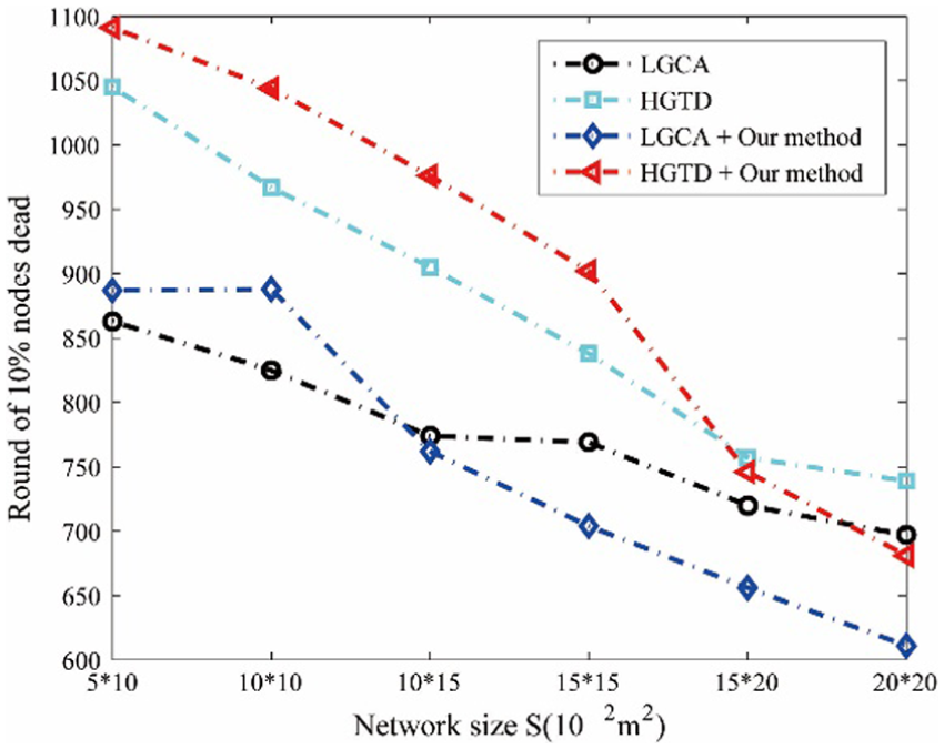
Comparison of rounds until 10% of the nodes die among LGCA, HGTD and their improved versions for several sizes of the network.
The network lifetime is a very important metric for the performance evaluation of the clustering protocols since it gives the moment when the network nodes begin to die. In addition, the lifespan of the last dead node is also important. Figure 18 shows a comparison of rounds until the last node dies among the four protocols for different sizes of the network. The improved LGCA has fewer rounds than the original LGCA in finishing its work (until the last node dies). In addition, the energy is used evenly in the improved version. The improved HGTD is almost the same as its original version in terms of the death of the last node, which indicates that all of the nodes in the improved HGTD can evenly use their energy and can effectively work in the network.

Comparison of rounds until the last node dies among LGCA, HGTD and their improved versions for several sizes of the network.
To show the performances of the improved protocols in detail, Figure 19 gives the number of alive nodes in each round for each of the four protocols when S = 1×10⁴ m2. It is clear that the improved LGCA has a shorter interval than its original version from the death of the first node to the last node, which indicates that the energy consumption among the nodes is well allocated in the improved LGCA but not in the original. At the same time, both HGTD and its improved version have shorter intervals. It is clear that both improved versions significantly outperform their original in terms of the first node dead and the last node dead.

Number of nodes alive versus rounds for LGCA, HGTD and their improved versions when S = 1 × 10⁴ m2.
Conclusion
In the cluster formation phase, the normal nodes’ allocation becomes important to the energy balance of the CHs. However, in earlier work, it depends only on some simple methods, which seriously affect the energy balance of the CHs and further degrade the performance of the whole WSN. Additionally, the number and distribution of the CHs are also important in our approach. If the distribution of the CHs is uneven, then the uncovered node(s) by any cluster will be selected as new CH(s) to attain a high coverage rate. Moreover, the number of CHs in a monitoring region is also restricted. Finally, a game-based, energy-balance method is proposed to apply in the cluster-based routing protocols for improving the WSNs’ performance. We select two clustering protocols, LGCA and HGTD, to compare with their improved versions combined with our method. The simulation shows that the improved protocols achieve better performance. In the future, we will apply the GT to analyse the multi-hop interest situation.
Footnotes
Appendix
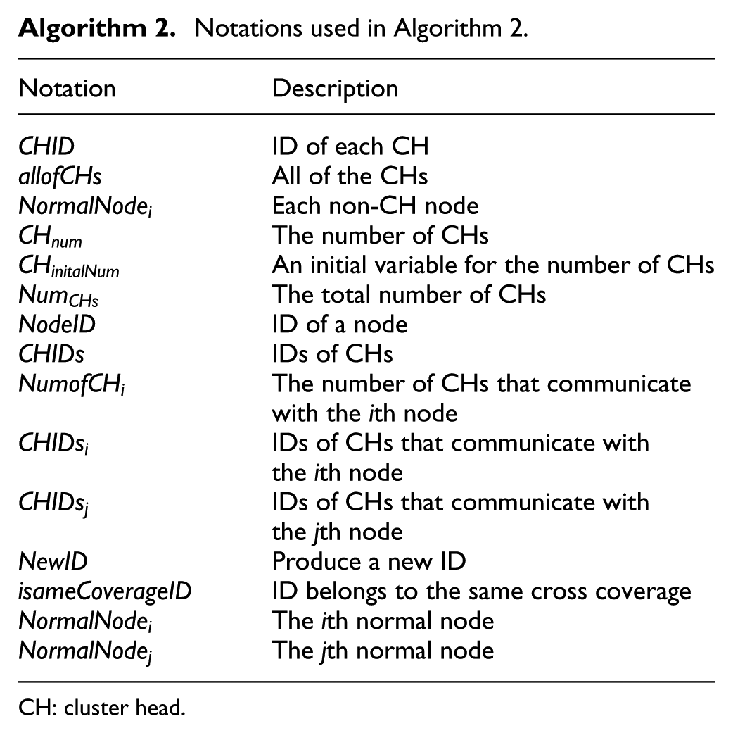
Notations used in Algorithm 2.
| Notation | Description |
|---|---|
| ID of each CH | |
| All of the CHs | |
| Each non-CH node | |
| The number of CHs | |
| An initial variable for the number of CHs | |
| The total number of CHs | |
| ID of a node | |
| IDs of CHs | |
| The number of CHs that communicate with the ith node | |
| IDs of CHs that communicate with the ith node | |
| IDs of CHs that communicate with the jth node | |
| Produce a new ID | |
| ID belongs to the same cross coverage | |
| The ith normal node | |
| The jth normal node |
CH: cluster head.
Academic Editor: Thomas Wettergren
Declaration of conflicting interests
The author(s) declared no potential conflicts of interest with respect to the research, authorship, and/or publication of this article.
Funding
The author(s) disclosed receipt of the following financial support for the research, authorship, and/or publication of this article: This work was supported by Project Supported by Scientific and Technological Research Program of Chongqing Municipal Education Commission (Grant No. KJ15012001), Fundamental Research Funds for the Central Universities in China (Grant No. 106112015CDJRC161203), Chongqing Postdoctoral Special Funding Project (Grant No. Xm2015063) and Major Program of National Natural Science Foundation of China (Grant Nos 61472053, 91438104 and 91420102).