Sage Journals: Discover world-class research

Abstract

Short-term traffic flow forecasting is a difficult yet important problem in intelligent transportation systems. Complex spatiotemporal interactions between the target road segment and other road segments can provide important information for the accurate forecasting. Meanwhile, spatiotemporal variable selection and traffic flow prediction should be solved in a unified framework such that they can benefit from each other. In this article, we propose a novel sparse hybrid genetic algorithm by introducing sparsity constraint and real encoding scheme into genetic algorithm in order to optimize short-term traffic flow prediction model based on least squares support vector regression. This method can integrate spatiotemporal variable selection, parameter selection as well as traffic flow prediction in a unified framework, indicating that the “goodness,” that is, contribution, of selected spatiotemporal variables and optimized parameters directly depends on the final traffic flow prediction accuracy. The real-world traffic flow data are collected from 24 observation sites located around the intersection of Interstate 205 and Interstate 84 in Portland, OR, USA. The experimental results show that the proposed sparse hybrid genetic algorithm-least square support vector regression prediction model can produce better performance but with much fewer spatiotemporal variables in comparison with other related models.

Keywords

Traffic flow forecasting spatiotemporal variable selection genetic algorithm road traffic network machine learning

Introduction

Intelligent transportation system (ITS)¹ which incorporates information and communication technology into traffic infrastructure and vehicles, has been applied to extenuate the traffic pressure, reduce fuel consumption, and improve environment quality in large cities. As an indispensable part of ITS, short-term traffic flow forecasting, defined to be predicting traffic flows at a target road site in the next time interval (usually in the range of 5–30 min), can be applied to traffic signal control, congestion alleviation, route guidance, adaptive ramp metering, and so on. For example, with the aid of reliable forecasting data, traffic managers are able to early realize the potential danger in unstable traffic condition and adopt necessary measures to ensure normal traffic operation. For travelers, they can receive the real time and dynamically estimated results about future traffic condition and make a decision on departure time or adjust travel routes before jam formation. Thus, short-term traffic forecasting has become an interesting topic and attracts more and more interests of researchers because of the significant role and wide range of applications in ITS. Nowadays, some traffic flow forecasting systems have been deployed in some ITS,² such as the Sydney Coordinated Adaptive Traffic System and parallel-transportation management systems.

Generally speaking, traffic flow forecasting can be regarded as a learning problem. A forecasting model is first constructed by learning the underlying variation patterns from the given historical traffic flow data and then used to forecast future situations based on real-time traffic variables. A traffic flow forecasting model generating estimation which is very consistent with actual traffic flow data is more preferable and valuable in real-world applications. Over the past decade, various traffic flow forecasting methods have been proposed.³ Accurate and reliable traffic flow forecasting, however, is still a challenging issue because traffic system is a highly nonlinear, time-variant, stochastic, and complex system.⁴

Some investigations in the literatures treat historical traffic flow for the target site as a time series process. They employ time series analysis theory to model the temporal variation of traffic flow and forecast the future trends. Some typical models include Kalman state space filtering models,^5–7 autoregressive integrated moving averaging (ARIMA),⁸ seasonal ARIMA (SARIMA),^9,10 k-nearest neighbor,¹¹ ridge regression,¹² and so on. These methods mainly characterize the temporal correlation of traffic flow at a specific location and perform well when the traffic variations are relatively stable. However, traffic flow forecasting is essentially a complex, nonlinear problem¹³ since the traffic flows at different locations may interact with each other. For instance, traffic flow at the target site will be intensively influenced by its adjacent sites, especially upstream traffic. Moreover, traffic flows from distant but correlated sites also have impact on the target site to a certain extent.¹⁴ As a result, merely utilizing the limited information about the target site may be insufficient for high accurate traffic flow prediction under unstable traffic conditions and complex road settings.³

Recently, constructing forecasting models that can incorporate information of more road locations or even the whole traffic network is increasingly drawing the attention from many researchers. Hobeika and Kim¹⁵ used current traffic, historical average, and upstream traffic to perform short-term traffic flow prediction. Sun et al.¹³ took into account the historical data from both current and upstream adjacent road segments in the Bayesian network framework. Min and Wynter¹⁶ predicted traffic flow by considering the spatial characteristics of a road network, including the distance and the average speed of the upstream road segments. Xu et al.¹⁷ first applied multivariate adaptive regression splines (MARS) model¹⁸ to identify most predictive variables which are then used to construct prediction model. Kamarianakis et al.¹⁹ divided the traffic flow into homogeneous regimes and applied l₁-norm penalized regression²⁰ in each regime to perform estimation and model selection simultaneously. Gao et al.²¹ applied graphical Lasso (least absolute shrinkage and selection operator)²² to select the most informative variables for traffic flow prediction. These methods exploit both temporal and spatial information among multiple road sites in terms of the variation of traffic flow, thus usually leading to better performance. However, the models are relatively complex and include many parameters which are difficult to adjust.

Because the rapid process change underlying traffic flow is too complicated to be captured by a single linear statistical model, various advanced machine learning methods, such as artificial neural network (ANN) and support vector machine (SVM), have been used to learn inherent regularity from historical traffic data for traffic flow forecasting. ANN is widely used in traffic flow forecasting, especially deep learning^23–25 because it is able to approximate any complex function without prior knowledge of the problem. Although ANN is a powerful nonlinear modeling tool, it has some limitations, such as the difficulty to interpret the involved black-box operations, the determination of suitable network structure including the number of hidden layers and neurons.

As a competing method, SVM²⁶ introduced by Vapnik and colleagues is another important machine learning method which has achieved great success in many real-world applications, including drug discovery,²⁷ robust regression,²⁸ pattern classification,²⁹ time series prediction,³⁰ and so on. In comparison with ANN, SVM has several remarkable advantages. First, it is based on structural risk minimization (SRM) principle³¹ which strikes a balance between traditional empirical risk and model complexity. Second, it can be used to solve nonlinear problems by kernel trick which means the input space is first mapped into a much higher (or even infinite) dimensional feature space wherein a linear SVM model is constructed. Third, SVM boils down to a quadratic programming (QP) problem³² which is convex and has globally optimal solution. The original SVM was developed to solve pattern classification problems. With the ε insensitive loss function introduced by Vapnik, SVM can be extended to solve nonlinear regression problems, namely, support vector regression (SVR). Furthermore, least squares SVR (LSSVR)³³ and its kernel version simplify traditional SVR by changing ε insensitive loss function into least squares loss function. In such a way, the solution of LSSVR can be found by solving a linear system of equations instead of complex QP problem, without sacrificing generalization performance. SVR and LSSVR are broadly exploited in traffic flow forecasting.^34–37

Although LSSVR can well model the inherent nonlinear relationship between historical data and future data, it has two main limitations. The first one is parameter optimization problem. The forecasting performance of LSSVR varies broadly with different combination of kernel width parameter $σ$ and regularization parameter $γ$ . As a result, without suitable combination of parameters, LSSVR may yield poor performance. The second issue is variable selection problem. LSSVR tries to use all of the input variables to construct nonlinear forecasting model. As a result, it is unable to select small number of crucial variables from original variable set and thus lacks interpretability. Moreover, training an LSSVR model directly on the data with excessive redundant and noisy variables will increase the complexity of model, thus possibly leading to the problem of overfitting and affecting the model performance to some extent.

Some works have focused on the parameter selection problem of LSSVR/SVR in traffic flow prediction. For example, Hong et al.³⁴ presented a short-term traffic flow forecasting model which uses continuous ant colony optimization (ACO) algorithm to adjust parameters in SVR. Zhang et al.³⁵ applied genetic algorithm (GA) to optimize the parameters in SVR for ship traffic flow prediction. Cong et al.³⁶ developed an LSSVR-based traffic flow forecasting model in which the fruit fly optimization algorithm (FOA) is applied to determine two parameters. Instead of FOA algorithm, Yusof et al.³⁷ used firefly algorithm (FA) to optimize the parameters of LSSVR. Overall, these works attempt to use different intelligent optimization algorithms, such as GA,³⁵ ACO,³⁴ to automatically determine suitable parameters for LSSVR/SVR.

However, the application of intelligent optimization algorithm for variable selection in the case of traffic flow forecasting is rare. Actually, variable selection is of great importance in constructing model for forecasting traffic flow data because the number of variables is generally much large, especially when simultaneously taking into account temporal and spatial information of the whole road network. For example, given a road network containing 24 sites and four time lags (i.e. four historical time points), the number of spatiotemporal variables involved in LSSVR reaches 120. Considering the topological structure of road network, the spatiotemporal variables collected at different time intervals and locations are actually closely related, thus making many variables highly correlated with each other or irrelevant with the traffic flow at the target site. It indicates that not all of these spatiotemporal variables are predictive or informative in terms of traffic flow forecasting at target site.^19,21 Directly fitting an LSSVR model to the traffic data including much redundant and/or noisy information will dramatically increase the complexity of forecasting model. Consequently, it may lead to overfitting and thus influence the effectiveness of model. In addition, lacking of variable selection ability also makes the resulting forecasting model difficult to interpret in the sense that it is hard to identify which spatiotemporal variables really contribute to the traffic flow prediction for the target site.

Motivated by the above discussions, in this article, we propose a novel traffic flow forecasting model by simultaneously dealing with the parameter selection and variable selection problems of LSSVR. A sparse hybrid genetic algorithm (SHGA) is developed to achieve this goal. Specifically, we first propose a hybrid encoding scheme of the chromosome, which can encode candidate parameters and variable subset, respectively, using real numbers and binary numbers. A sparsity constraint is further imposed on the binary encoding in order to restrict the number of variables involved in LSSVR. An elaborately designed crossover and mutation strategies finely tuned for the above hybrid encoding scheme is presented to implement the evolution of population. In such a way, it is possible to find sparse optimal solution for general optimization problems. We apply the SHGA to optimize traffic flow forecasting model based on LSSVR and present the whole flowchart. In such a way, we can not only determine the suitable combination of kernel width parameter $σ$ and regularization parameter $γ$ , but also fully excavate crucial information contained in the road network by selecting few spatiotemporal variables. To evaluate the effectiveness of the proposed method, real-world traffic flow data are collected from 24 observation sites spreading over two freeways called I84 and I205 which cross with each other in Portland, OR, USA. The experimental results show that the proposed traffic flow model can achieve better forecasting accuracy but with much fewer spatiotemporal variables in comparison with other methods.

The rest of this article is organized as follows. Section “Preliminaries” describes the preliminaries, including the definition of short-term traffic flow forecasting problem and an overview of LSSVR. Section “Model description” presents the proposed joint spatiotemporal variable and parameter selection method. Section “Experiments and analysis” presents the road network traffic data, extensive experiments, and detailed results analysis. Finally, we draw some conclusions in section “Conclusion.”

Preliminaries

Problem definition

Consider a road network consisting of $N$ sites which are equipped with traffic sensors (e.g. loop detectors). Assume that at given time interval $t$ (e.g. every 15 min), the sth site provides a traffic data reading $v_{s} (t)$ (e.g. volume or speed). Then, the short-term traffic flow forecasting problem can be formulated as follows.

Given a set of historical and current readings $X = {v_{s} (t), v_{s} (t - 1), \dots, v_{s} (t - lag) | s = 1, 2, \dots, N} \in R^{P}$ , where $t$ represents the current time, $lag$ denotes the time lag, $s$ denotes the site, $P = N \times (lag + 1)$ is the total number of variables. Obviously, $X$ is able to characterize the current and previous traffic state of the whole road network. In this article, each element in $X$ is called spatiotemporal variable since it is determined by time and geography. The goal of short-term traffic flow forecasting is to predict $Y = v_{s} (t + h)$ for an arbitrary site $s$ , where $h \geq 1$ denotes the prediction horizon. For instance, $h = 1$ refers to the prediction of traffic flow at $t + 1$ based on the current and historical data.

Least squares SVR

Given a set of training samples denoted as ${x_{i}, y_{i} | i = 1, 2, \dots, M}$ where $x_{i} \in R^{N \cdot (lag + 1)}$ is an input vector consisting of $P$ spatiotemporal variables, $y_{i} \in R$ is the corresponding response variable (traffic flow at the target site), and $M$ is the total number of samples. The goal of LSSVR³³ is to construct a mapping function from the input $x$ to the output $y$ : $f (x) \to y$ , such that $f (x)$ can yield good estimation for future $x$ which is outside the training set. This mapping function is usually parameterized as

f (x) = w^{T} φ (x) + b

(1)

where $w$ and $b$ are called weight vector and bias, respectively, $φ (x)$ is a predefined nonlinear kernel function mapping the input space to a new high (or even infinite) dimensional feature space. By such mapping, it is possible to convert the complex nonlinear relationship between $x$ and $y$ into a simple linear relationship between $φ (x)$ and $y$ as shown in equation (1). To find the desired $w$ and $b$ , we need to solve the following LSSVR objective function^33,38

\min \frac{1}{2} w^{2} + \frac{1}{2} γ \sum_{i = 1}^{M} e_{i}^{2}

(2)

s . t . w^{T} φ (x_{i}) + b - y_{i} = e_{i}

where $e_{i}$ is the estimation error between the predicted value and actual value, $γ$ is a trade-off parameter, responsible for balancing the model complexity and estimation error. To solve the above optimization problem, we introduce the corresponding Lagrange function as follows

\begin{array}{l} L (w, b, e_{i}, α_{i}) = \frac{1}{2} w^{2} + \frac{1}{2} γ \sum_{i = 1}^{M} e_{i}^{2} \\ - \sum_{i = 1}^{M} α_{i} (w^{T} φ (x_{i}) + b - y_{i} - e_{i}) \end{array}

(3)

where $α_{i}$ denotes Lagrange multiplier. To find the optimal solution, we exploit the well-known Karush–Kuhn–Tucker conditions³² and get the following equations

{\begin{matrix} \frac{\partial L}{\partial w} = w - \sum_{i = 1}^{M} α_{i} φ (x_{i}) = 0 \\ \frac{\partial L}{\partial b} = - \sum_{i = 1}^{M} α_{i} = 0 \\ \frac{\partial L}{\partial e_{i}} = γ e_{i} + α_{i} = 0 \\ \frac{\partial L}{\partial α_{i}} = - (w^{T} φ (x_{i}) + b - y_{i} - e_{i}) = 0 \end{matrix}

(4)

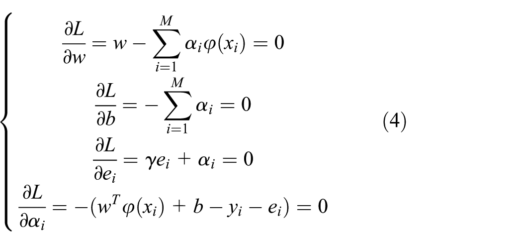
By simplifying the above equations, we can get the following linear system of equations

[\begin{matrix} K + \frac{I}{γ} & 1 \\ 1^{T} & 0 \end{matrix}] (\begin{matrix} α \\ b \end{matrix}) = (\begin{matrix} y \\ 0 \end{matrix})

(5)

where $K$ is a $M \times M$ kernel matrix with element $K_{ij} = K (x_{i}, x_{j}) = φ (x_{i})^{T} φ (x_{j})$ , 1 is a vector of ones, I is an identity matrix of appropriate dimensions. After solving equation (5) to obtain $α$ and $b$ , we can get the prediction function $f (x)$ as

f (x) = \sum_{i = 1}^{M} α_{i} K (x_{i}, x) + b

(6)

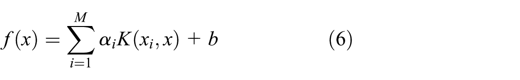
Kernel function plays an important role especially when solving nonlinear problems based on LSSVR model. In this article, we use Gaussian kernel as follows

K (x_{i}, x_{j}) = \exp {(- \frac{(x_{i} - x_{j})}{σ^{2}})}^{2}

(7)

where $σ$ is the width parameter of kernel function. Gaussian kernel is used in numerous traffic flow forecasting problems owing to its convenient implementation and powerful nonlinear modeling ability.

As can be seen, on one hand, the performance of LSSVR performance depends on the combination of its some vital parameters such as the trade-off parameter $γ$ and kernel width parameter $σ$ . For instance, large $γ$ tends to reduce the training error, thus may lead to overfitting. In contrast, small $γ$ will reduce the model complexity, but may lead to underfitting. Similarly, large $σ$ prefers a more flat Gaussian function and easily results in underfitting while small $σ$ makes the Gaussian function more sharp and may cause overfitting. Without a proper combination of these parameters, LSSVR will fail to keep good forecasting performance. Thus, parameter selection for $γ$ and $σ$ is necessary and crucial for the application of LSSVR.

On the other hand, as can be seen from Gaussian kernel (7), all variables in $x_{i} \in R^{P}$ equally take part in the calculation of kernel matrix, without distinguishing their respective significance. In the case of road network traffic flow forecasting, $x_{i}$ which summaries the current and historical state of the whole road network usually has a high dimensionality and many elements may be correlated to each other or irrelevant to the response variable $y_{i}$ . As a result, making use of those redundant or irrelevant spatiotemporal information will inevitably influence the calculation of kernel matrix and in turn affect the performance of traffic flow forecasting. Moreover, it also makes the resulting model difficult to interpret, that is, which spatiotemporal variables really contribute to forecasting the traffic flow at the target site. Therefore, spatiotemporal variable selection is also an important and interesting issue for the application of LSSVR to traffic flow forecasting.

Model description

Genetic algorithm

GA³⁹ is a heuristic search algorithm aiming to solve the optimization problem. It was originally developed from some phenomena in evolutionary biology, including genetics, mutation, natural selection, and hybridization. This method is very flexible and attractive, especially suitable for optimization problems without explicit objective function and/or difficult to solve using traditional numeric algorithms, for example, gradient descent.

To solve an optimization problem, GA first generates a population with an abstract representation of many candidate solutions. Traditionally, a solution can be represented in the form of chromosome (or called chromosome) which comprises multiple genes. The commonly used representation method is binary encoding, that is, 0 and 1 although some other representation methods are also available, such as real encoding.⁴⁰ Evolution begins with the population with completely random chromosomes. All chromosomes in the current population are evaluated by a predefined fitness function and then a certain number of superior chromosomes are preserved according to their fitness values and some selection strategy. Favorable chromosomes have more chance to be selected while unfavorable chromosomes are less likely to survive. Afterwards, crossover and mutation operations are applied on those preserved chromosomes in order to generate offspring in a new population. By doing so, the population as a whole can evolve toward better solutions. After many iterations, the chromosomes with favorable fitness will dominate the population and yield solutions which are good enough for the optimization problem.

Sparse hybrid GA with LSSVR

In this section, we propose a sparse hybrid GA which can implement simultaneous spatiotemporal variable and parameter selection automatically in LSSVR for effective traffic flow forecasting. The details of this method are explained as follows.

Chromosome representation

The first step when applying GA is to represent each candidate solution by a chromosome in population. To achieve joint spatiotemporal variable and parameter selection for traffic flow forecasting, we design a chromosome representation by combining real encoding and binary encoding in a unified scheme. This chromosome representation method is illustrated in Figure 1 where each element in chromosome $V$ is called gene. As can be seen, each chromosome consists of two parts. The left part in Figure 1 uses two real encoding genes (or parameter genes) to represent different combinations of parameters $γ$ and $σ$ . The two real parameters are restricted in the range of $[V_{\min}, V_{\max}]$ where $V_{\min}$ and $V_{\max}$ are two predefined constants, referring to the minimum and maximum values allowed for parameter genes. The right part in Figure 1 uses binary encoding genes (or variable genes) to define whether the associated spatiotemporal variables should be chosen to train the LSSVR model. Here, the location of “1” in binary encoding means the corresponding variable should be preserved, while the location of “0” means the variable should be removed from the final forecasting model. It is obvious that each chromosome in this representation is comprised of totally $2 + P$ genes.

Figure 1.

An illustration of chromosome representation.

Furthermore, in order to restrict the number of spatiotemporal variables fed into LSSVR model, we require the binary encoding genes across all chromosomes in the population that have the same number of “1,” which is usually very small in comparison with the total number of variables. This imposed sparsity can guarantee very few spatiotemporal variables which really contribute to forecasting the traffic flow at the target site can be well selected. To sum up, this chromosome representation method has two interesting characteristics. One is that it is made up of both parameter genes and variable genes which use different encoding schemes. The other is that the number of variable genes marked as “1” is restricted in order to control the sparsity of variable selection.

Fitness function

Fitness function is regarded as an important component in GA, responsible for estimating the quality of each chromosome in current population. In this work, the root mean squared error (RMSE), which is widely used to evaluate the performance of traffic flow forecasting models, acts as the fitness function. Thus, smaller fitness value indicates better chromosome. Specifically, given a validation data set ${(x_{1}, y_{1}), (x_{2}, y_{2}), \dots, (x_{M'}, y_{M'})}$ , $M'$ is the number of validation samples, the RMSE can be calculated as follows

RMSE = \sum_{i = 1}^{M'} (y_{i} - {\hat{y}}_{i})^{2}

(8)

where $y_{i}$ and ${\hat{y}}_{i}$ are the actual value and the predicted value for ith validation sample, respectively. Note that besides RMSE, mean absolute error (MAE) is also widely used. The two metrics are generally consistent with each other. However, in some cases where large outliers occur, MAE may be a better choice. For the current problem, outliers seldom occur. Thus, we used RMSE as fitness function.

Selection, crossover, and mutation

Some chromosomes need to be selected from the current population to be parents. According to Darwin’s evolution theory, the superior ones should survive and create new offspring. In this work, half of the current population are kept following rank selection principle³⁹ which can guarantee that all the chromosomes have a chance to be selected.

These selected chromosomes are randomly matched to form parent pairs and then the crossover operator is conducted so as to generate child chromosomes. Suppose the probability of crossover is $pc$ . Since the chromosome is made up of different types of genes (parameter genes and variable genes), we have to design different crossover operator according to their specific properties.

For real encoding, the parameter genes in child chromosomes can be expressed by the linear combination of the corresponding parent chromosomes as follows

{\begin{matrix} V_{1}^{c} (i) = α V_{1}^{p} (i) + (1 - α) V_{2}^{p} (i) \\ V_{2}^{c} (i) = β V_{1}^{p} (i) + (1 - β) V_{2}^{p} (i) \end{matrix} i = 1, 2, if rand > pc

(9)

where $rand$ denotes a randomly generated number, $V_{1}^{p} (i)$ and $V_{2}^{p} (i)$ are the parameter genes in parent chromosomes, $V_{1}^{c} (i)$ and $V_{2}^{c} (i)$ are the parameter genes in child chromosomes, and $α$ and $β$ are two random numbers uniformly distributed on the interval $[- 0.25, 1.25]$ .

For the binary encoded variable genes, we attempt to keep the number of “1” in the chromosome unchanged after crossover operation so as to keep the imposed sparsity consistent across all newly generated chromosomes. Therefore, we propose a multi-point crossover operator for variable genes. Specifically, define two index sets as $A = {i | V_{1}^{p} (i) = 0 \land V_{2}^{p} (i) = 1, i = 3, 4, \dots, P}$ and $B = {i | V_{1}^{p} (i) = 1 \land V_{2}^{p} (i) = 0, i = 3, 4, \dots, P}$ . Then, the variable genes in child chromosomes are given by

{\begin{matrix} V_{1}^{c} (j) = 1, V_{2}^{c} (j) = 0, j \in \hat{A} \subset A \\ V_{1}^{c} (j) = 0, V_{2}^{c} (j) = 1, j \in \hat{B} \subset B \end{matrix} if rand > pc

(10)

where $\hat{A}$ and $\hat{B}$ are two randomly generated subsets of $A$ and $B$ , respectively, and they have the same number of elements. An illustration of the crossover operator is shown in Figure 2.

Figure 2.

An illustration of chromosome crossover operator.

Similarly, we need to construct different mutation strategies for different types of genes. In this study, for real encoded parameter genes, we randomly replaced the original value with a new value in the range of $[V_{\min}, V_{\max}]$ . This is expressed as

V (i) = β (V_{\max} - V_{\min}) + V_{\min}, if rand > pm, i = 1, 2

(11)

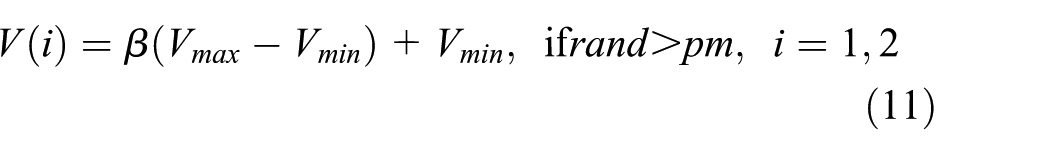
where β is a random number distributed in [0,1] and $pm$ is a very small mutation rate.

For binary encoded variable genes, a “1” at arbitrary location is replaced with “0.” Meanwhile, a “0” at arbitrary location is replaced with “1.” In such a way, we can not only keep the number of variable genes with value “1” (and also “0”) constant, but also achieve the goal to enrich the diversity for population.

Framework

The flowchart of our proposed SHGA-LSSVR method for short-term traffic flow forecasting is shown in Figure 3. An explanation is described as follows:

Step 1. Collect traffic flow data from real-world road network equipped with loop detectors, which are partitioned into training, validation, and testing data.

Step 2. Perform normalization on the data to have zero mean and standard deviation.

Step 3. Initialize GA population by randomly generating binary encoded genes and real encoded genes.

Step 4. Construct multiple LSSVR models, based on training data and chromosomes in population, and then evaluate fitness of each model on validation data.

Step 5. If GA does not converge, go to Step 6, otherwise go to Step 7.

Step 6. Execute selection, crossover, and mutation operations based on current population to generate updated population, then go to Step 4.

Step 7. Pick up optimal chromosomes and identify the selected variables and optimal parameters.

Step 8. Construct the final LSSVR model based on variable subset and optimal parameters.

Step 9. Apply LSSVR on the testing data to generate forecasting results.

Figure 3.

Flowchart of SHGA-LSSVR for traffic flow forecasting.

Experiments and analysis

Data description

In this article, we use the traffic flow data collected by loop detectors installed at 24 observation sites. These sites are located around the intersection of Interstate 205 (I205) and Interstate 84 (I84) in Portland, OR, USA. The data can be downloaded from the website (http://portal.its.pdx.edu/). The locations of these 24 sites and their numbers are labeled on the sub-area map of Portland shown in Figure 4. Overall, 18 sites locate on the I84 and 6 sites locate on the I205. Each site is denoted by a solid circle with different colors. Black indicates the traffic flow from west to east and green represents the opposite direction. Similarly, red indicates the traffic flow from north to south and purple represents the opposite direction. We use the 15 min aggregation data whose unit is vehicles per 15 min (veh/15 min). Therefore, there are totally 96 sample points for each site and every day. We collect traffic flow data of 10 weekdays (from 18 September to 1 October 2015) of each site and discard the data belonging to holidays and weekends because the traffic states on weekends and holidays vary differently from the weekdays. Furthermore, in order to train various models, choose their parameters and evaluate the prediction performance of models, we split the whole data set into three parts. The first eight weekdays of 18–29 September (by removing weekends and holidays) are grouped as the training set, the data set of 30 September is regarded as the validation set and the data set of 1 October is treated as the test set. In our experiments, we chose six sites (3, 10, 12, 19, 21, and 24) as the target sites that we want to forecast. These target sites are intentionally labeled with yellow in Figure 4 for clear illustration of their distribution in the road network.

Figure 4.

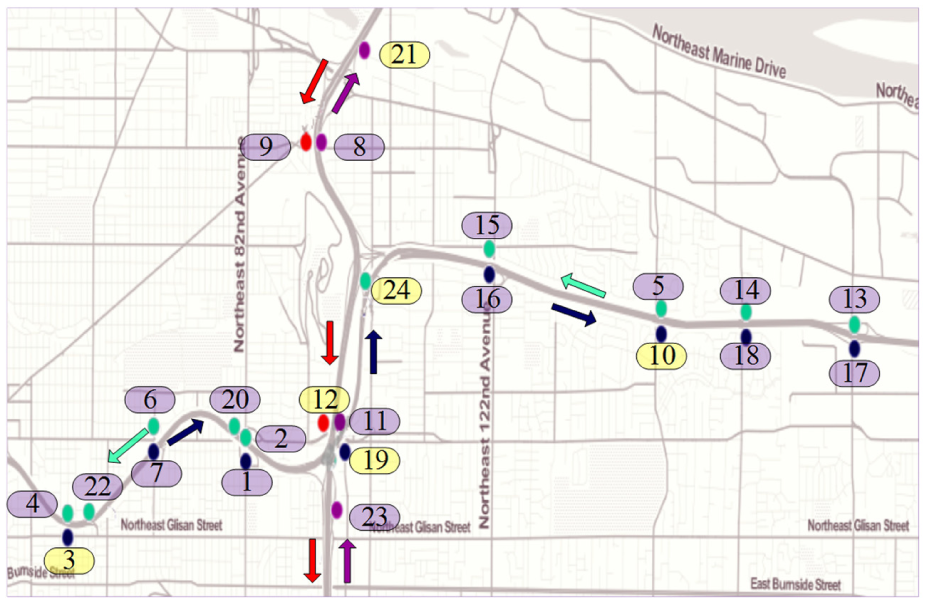
The selected sub-area road network of Portland, OR, USA.

Due to the malfunction of some detectors or transmission errors, there exist some missing values in the original traffic flow data. We count the ratio of missing values to total values and find that the missing rate (<1% for) is very small for these sites and time range. Since our model is not applicable in case of missing values, a simple temporal correlation based traffic flow imputation method is applied to complete these missing values.

Configuration

In order to evaluate the effectiveness of the proposed SHGA-LSSVR method for short-term traffic flow forecasting, we conduct extensive experiments based on the above real-world traffic data set. We compare SHGA-LSSVR with three closely related methods, including Ridge regression, Lasso regression,²⁰ and the original LSSVR without variable selection. Ridge and Lasso share the same least squares loss function; however, they have different penalty terms. In particular, Ridge is penalized by the l₂-norm of model parameters, while Lasso is penalized by the l₁-norm of model parameters. Due to such subtle but important difference, Lasso can achieve variable selection as the proposed SHGA-LSSVR while Ridge cannot. In addition, it should be emphasized that Ridge and Lasso are both linear regression models. LSSVR with Gaussian kernel is also involved in our experiments because of its powerful nonlinear modeling ability as well as wide applications in time series forecasting. In this study, the parameters in all methods are selected based on grid search and prediction error on the validation traffic flow data. All methods are implemented in MATLAB environment on a PC with Intel(R) Core i7 3.5 GHz with 16 GB RAM. The SHGA-related parameters for the proposed model are shown in Table 1.

Table 1.

Parameters for SHGA.

Parameter	Value
Population size	20
$V_{\min}$	0.0073
$V_{\max}$	512
$pc$	0.8
$pm$	0.03
Number of iteration	100

SHGA: sparse hybrid genetic algorithm.

To compare the prediction performance of various forecasting methods, two widely used criteria, namely, RMSE and mean absolute percentage error (MAPE),¹⁷ are adopted in this study. In addition, since Lasso and our SHGA-LSSVR both can select spatiotemporal variables, the number of selected variables is also recorded which indicates the prediction performance can be achieved with typically much fewer variables. Taking into account the influence of different time lags on prediction performance, we change the time lags from 1 to 5 and record the experimental results for each case. The correspondence between time lag and the total number of spatiotemporal variables is shown in Table 2. For example, when time lag equals 1, the traffic flow data collected at time $t$ and $t - 1$ from all 24 sites are used to predict the traffic flow at the target site at time $t + 1$ . Thus, it generates totally 48 spatiotemporal variables in this case.

Table 2.

Correspondence between time lag and the number of spatiotemporal variables.

Time lag	1	2	3	4	5
#variables	48	72	96	120	144

Prediction error analysis

First, we take site 21 as an example to analyze different methods. The prediction errors in terms of RMSE and MAPE criterion obtained by all the methods under different time lags are listed in Table 3. From these experimental results, some interesting observations can be summarized as follows.

Table 3.

RMSE of different prediction methods on site 21.

Method	lag = 1		lag = 2		lag = 3		lag = 4		lag = 5
Method	RMSE	MAPE	RMSE	MAPE	RMSE	MAPE	RMSE	MAPE	RMSE	MAPE
Ridge	96.35	19.64	93.01	17.95	93.42	18.62	91.75	17.85	90.99	17.98
Lasso	94.50	17.25	91.75	16.81	92.53	17.71	92.56	17.75	90.09	16.75
LSSVR	87.90	11.53	90.56	12.30	86.21	12.80	87.36	13.52	86.41	13.28
SHGA-LSSVR	79.69	11.33	82.91	11.27	83.13	11.75	79.73	11.41	79.12	11.36

RMSE: root mean squared error; MAPE: mean absolute percentage error; SHGA: sparse hybrid genetic algorithm; LSSVR: least squares support vector regression.

Significance of bold values are the best results.

For Ridge and Lasso, which are two linear methods, we can see their performance is worse than two nonlinear methods, LSSVR and SHGA-LSSVR. This is because the variation of traffic flow is actually very complex and highly nonlinear, especially in the case of road network where many potential factors may influence the prediction at the target site. Ridge and Lasso are more suitable when the relationship between the input and the output is approximately linear. Comparing LSSVR and SHGA-LSSVR, we can see the latter achieves smaller prediction error than the former. We have performed paired t-test at 5% significance level for the null hypothesis that the performance achieved by our proposed SHGA-LSSVR and other methods is the same. The results are shown in Table 4. As we can see from the results, in most cases, the proposed method outperforms the other competitors significantly.

Table 4.

Significance test of the proposed SHGA-LSSVR to other methods.

Method	lag = 1		lag = 2		lag = 3		lag = 4		lag = 5
Method	RMSE	MAPE	RMSE	MAPE	RMSE	MAPE	RMSE	MAPE	RMSE	MAPE
Ridge	<1e−3	<1e−3	<1e−3	<1e−3	<1e−3	<1e−3	<1e−3	<1e−3	<1e−3	<1e−3
Lasso	<1e−3	<1e−3	<1e−3	<1e−3	<1e−3	<1e−3	<1e−3	<1e−3	<1e−3	<1e−3
LSSVR	0.005	0.993	0.004	0.047	0.017	0.051	0.006	0.028	0.009	0.025

RMSE: root mean squared error; MAPE: mean absolute percentage error; SHGA: sparse hybrid genetic algorithm; LSSVR: least squares support vector regression.

For the computational time and execution time, we have reported the experimental results in Table 5. As can be seen, in terms of computational time, the proposed SHGA-LSSVR is slower than LSSVR because variable selection and parameter optimization are performed using GA, which is time-consuming. On the other hand, in terms of execution time, we found that SHGA-LSSVR is actually faster than LSSVR. This is reasonable since test can be performed based on those selected variables instead of all variables. Note that model training can be performed offline and execution time is usually an important factor for practical application of algorithm. As a result, the proposed method not only has superior prediction accuracy, but also less execution time, in comparison with original SVMs

Table 5.

Computational time (second) of each method.

Method	lag = 1		lag = 2		lag = 3		lag = 4		lag = 5
Method	Train	Test	Train	Test	Train	Test	Train	Test	Train	Test
Ridge	0.038	5.04e−05	0.047	2.73e−05	0.040	5.92e−04	0.056	3.33e−05	0.085	5.73e−05
Lasso	0.682	3.10e−04	0.901	3.14e−04	0.898	3.21e−04	1.295	3.65e−04	1.320	4.75e−04
LSSVR	49.83	0.0043	47.78	0.0066	51.20	0.0049	50.39	0.0112	50.48	0.0082
SHGA-LSSVR	246.07	0.0038	259.53	0.0045	267.87	0.0038	273.99	0.0029	281.34	0.0048

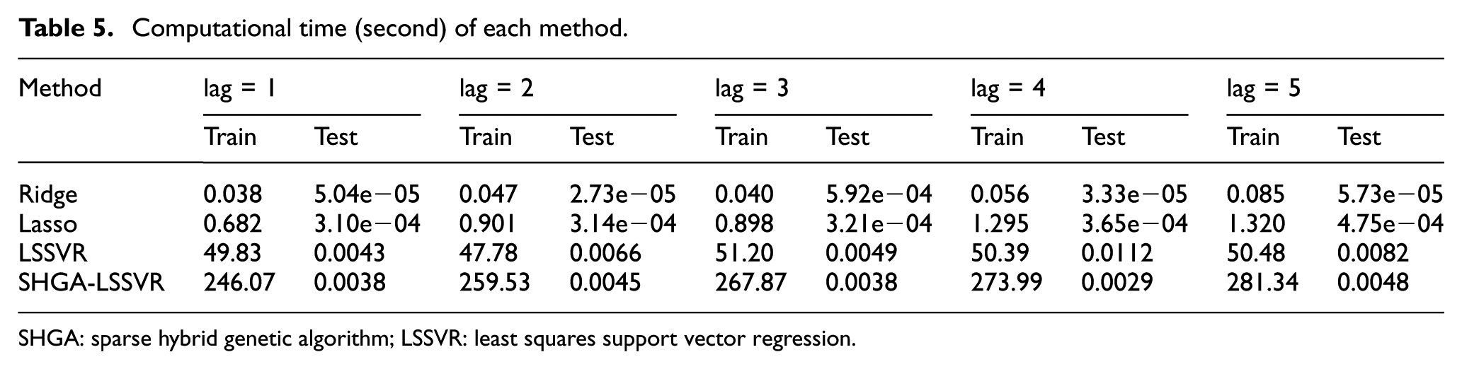
SHGA: sparse hybrid genetic algorithm; LSSVR: least squares support vector regression.

The number of spatiotemporal variables involved in each method is shown in Table 6. From the viewpoint of variable selection, Ridge and LSSVR are unable to select crucial variables, thus they use all available variables to construct the prediction model. In contrast, Lasso and the proposed SHGA-LSSVR can jointly choose a small number of variables from the whole set and construct the prediction method. However, as mentioned above, Lasso is a linear method, while SHGA-LSSVR is a nonlinear method. It enables SHGA-LSSVR to select fewer variables than Lasso and at the same time achieve better prediction performance because it can reveal the nonlinear relationship between those spatiotemporal variables.

Table 6.

Number of variables in different prediction models on site 21.

Method	lag = 1	lag = 2	lag = 3	lag = 4	lag = 5	Average
Ridge	48	72	96	120	144	96
Lasso	9	24	15	17	42	21.4
LSSVR	48	72	96	120	144	96
SHGA-LSSVR	20	12	14	14	16	15.2

SHGA: sparse hybrid genetic algorithm; LSSVR: least squares support vector regression.

To intuitively illustrate the prediction results of different methods, we show the actual traffic flow, the predicted traffic flow, and the associated residual obtained by each method in Figure 5. From these results, we can observe that the proposed SHGA-LSSVR achieves smaller prediction error than the other competitors, indicating this method can better capture the traffic flow pattern.

Figure 5.

Prediction results obtained by Ridge, Lasso, LSSVR, and SHGA-LSSVR.

For the other sites, that is, 24, 19, 3, 12, and 10, the experimental results including prediction RMSE, MAPE, and the number of spatiotemporal variables that are selected by SHGA are depicted in Figure 6. As we can observe, these results further verify that in most cases, the proposed SHGA-LSSVR outperforms all the other methods in terms of prediction error and at the same select fewer spatiotemporal variables.

Figure 6.

Prediction results comparison of different methods. From top row to bottom row: sites 3, 12, 19, 24, and 10.

Interpretation of spatiotemporal variables

An advantage of the proposed SHGA-LSSVR is its interpretability which can provide some useful insights about the spatiotemporal relationship between the selected spatiotemporal variables and the target site in terms of traffic flow forecasting. When the SHGA optimization is finished, the variable subset with superior performance can be obtained, implying that the resulting variables from the sites located in the same road network, contribute to the target site. In terms of the site 21 with 4 time lags, the selected 14 spatiotemporal variables from the totally 120 variables are shown in Figure 7. Specifically, the center large circle in Figure 7 represents the target site 21 to be predicted. The surrounding small circles with different size and color represent 120 spatiotemporal variables associated with 24 sites in the road network. The size of each circle indicates the time lag, that is, the larger the circle, the smaller the lag. For instance, the biggest circle for each site denotes 0 time lag and the smallest circle indicates 4 time lags. The color is used to differentiate 24 sites. The straight lines connecting the surrounding small circles and the center large circle indicate that these spatiotemporal variables contribute to the traffic flow prediction at the target site. Accordingly, these selected sites are marked by bisque in Figure 8. From these results, we can observe some interesting findings.

Figure 7.

Variable selection result for site 21 with 4 time lags.

Figure 8.

Distribution of the sites (bisque) related to target site 21.

On the whole, 10 sites are related to the target site 21 besides itself, which are 5, 7, 8, 11, 13, 14, 18, 19, 23, and 24. Among them, sites 8, 11, and 23 contribute to the target site 21 as the role of direct upstream sites. These sites all belong to I205. In addition, sites 5, 7, 13, 14, 18, 19, and 24 which locate on I84 also influence the traffic flow at the target site because I205 and I84 actually intersect and their traffic flows may impact each other. We also observe that for site 21, only the traffic flow immediately prior to the prediction time is selected, thus implying the inclusion of historical data of the target site is unnecessary. This observation is well consistent with Yang et al.¹⁴ In addition, many selected sites are not the nearest neighboring of the target site, reflecting that not only the adjacent sites but also the distant sites can have significant influence on the target site in the case of road network. This also coincides with the conclusion given in Yang et al.¹⁴ Generally speaking, the relationship between these spatiotemporal variables is rather complex. Nevertheless, the proposed SHGA-LSSVR method can automatically select only 14 variables from all 120 variables and at the same time construct an accurate prediction model for traffic flow forecasting.

Conclusion

In this article, we propose a novel SHGA optimized LSSVR model for road network short-term traffic flow forecasting. This method can combine spatiotemporal variable selection, hyperparameters optimization, and traffic flow prediction in a unified framework, indicating that the “goodness,” that is, contribution, of selected spatiotemporal variables and optimized parameters directly depends on the final prediction performance. In such a way, the spatiotemporal correlations among all other road segments and the target site are fully excavated and the parameters in LSSVR are also optimized simultaneously so as to improve the prediction performance. We exploit the real-world traffic flow data to evaluate the prediction ability of our proposed model. The experimental results show that in comparison with other methods, the proposed SHGA-LSSVR model can achieve better prediction performance with much fewer spatiotemporal variables. In the current work, we adopted LSSVR as prediction model because it has been widely used and shown promising results. However, it should be noticed that besides LSSVR, neural network based prediction models, such as deep learning,^23–25 have attracted much attention during the last few years. Comparing with LSSVR, deep learning is able to show better prediction accuracy given large number of samples. However, spatiotemporal variable selection has not been taken into account in current deep learning based prediction models. Therefore, the integration of the proposed SHGA with deep learning for further improvement of prediction is an interesting problem that we will investigate in the future work.

Footnotes

Acknowledgements

The authors would like to thank the anonymous reviewers for their constructive comments and suggestions.

Academic Editor: Michele Magno

Declaration of conflicting interests

The author(s) declared no potential conflicts of interest with respect to the research, authorship, and/or publication of this article.

Funding

The author(s) disclosed receipt of the following financial support for the research, authorship, and/or publication of this article: This work was partially supported by the National Natural Science Foundation of China (Grant Nos 61203244, U1564201, U1664258, 61601203, and 61403172), Fujian Provincial Key Laboratory of Information Processing and Intelligent Control (Minjiang University) (MJUKF201724), Key Research and Development Program of Jiangsu Province (BE2016149), Natural Science Foundation of Jiangsu Province (BK20140555), and the Talent Foundation of Jiangsu University, China (No. 14JDG066).

References

Zhang

Wang

. Data-driven intelligent transportation systems: a survey. IEEE T Intell Transp 2011; 12(4): 1624–1639.

Wang

FY.

Parallel control and management for intelligent transportation systems: concepts, architectures, and applications. IEEE T Intell Transp 2010; 11(3): 630–638.

Vlahogianni

Karlaftis

MG.

Short-term traffic forecasting: where we are and where we’re going. Transport Res C: Emer 2014; 43: 3–19.

Jin

Zhang

HM.

The inhomogeneous kinematic wave traffic flow model as a resonant nonlinear system. Transport Sci 2003; 37(3): 294–311.

Ojeda

Kibangou

Canudas de Wit

Adaptive Kalman filtering for multi-step ahead traffic flow prediction. In: Proceedings of the American control conference, Washington, DC, 17–19 June 2013. New York: IEEE.

Stathopoulos

Karlaftis

GM.

A multivariate state space approach for urban traffic flow modeling and prediction. Transport Res C: Emer 2003; 11(2): 121–135.

Guo

Huang

Williams

BM.

Adaptive Kalman filter approach for stochastic short-term traffic flow rate prediction and uncertainty quantification. Transport Res C: Emer 2014; 43: 50–64.

Williams

Multivariate vehicular traffic flow prediction: evaluation of ARIMAX modeling. Transp Res Record 2001; 1776(1): 194–200.

Lippi

Bertini

Frasconi

Short-term traffic flow forecasting: an experimental comparison of time-series analysis and supervised learning. IEEE T Intell Transp 2013; 14(2): 871–882.

10.

Kumar

Vanajakshi

Short-term traffic flow prediction using seasonal ARIMA model with limited input data. Eur Transp Res Rev 2015; 7: 21.

11.

Habtemichael

Cetin

Short-term traffic flow rate forecasting based on identifying similar traffic patterns. Transport Res C: Emer 2015; 66: 61–78.

12.

Haworth

Shawe-Taylor

Cheng

. Local online kernel ridge regression for forecasting of urban travel times. Transport Res C: Emer 2014; 46: 151–178.

13.

Sun

Zhang

A Bayesian network approach to traffic flow forecasting. IEEE T Intell Transp 2006; 7(1): 124–132.

14.

Yang

Shi

. Spatiotemporal context awareness for urban traffic modeling and prediction: sparse representation based variable selection. PLoS ONE 2015; 10(10): e0141223

15.

Hobeika

Kim

CK.

Traffic-flow-prediction systems based on upstream traffic. In: Proceedings of the vehicle navigation and information systems conference, Yokohama, Japan, 31 August –2 September 1994, pp.345–350. New York: IEEE.

16.

Min

Wynter

Real-time road traffic prediction with spatio-temporal correlations. Transport Res C: Emer 2011; 19(4): 606–616.

17.

Kong

Klette

. Accurate and interpretable Bayesian MARS for traffic flow prediction. IEEE T Intell Transp 2014; 15(6): 2457–2469.

18.

Friedman

JH.

Multivariate adaptive regression splines (with discussion). Ann Stat 1991; 19(1): 1–141.

19.

Kamarianakis

Shen

Wynter

Real-time road traffic forecasting using regime-switching space-time models and adaptive Lasso. Appl Stoch Model Bus 2012; 28(4): 297–315.

20.

Tibshirani

Regression shrinkage and selection via the Lasso. J R Stat Soc 1996; 58(1): 267–288.

21.

Gao

Sun

Shi

. Network-scale traffic modeling and forecasting with graphical Lasso. In: Liu

Zhang

Polycarpou

. (eds) Advances in neural networks—ISNN 2011. Berlin Heidelberg: Springer, 2011, pp.1358–1367.

22.

Friedman

Hastie

Tibshirani

Sparse inverse covariance estimation with the graphical Lasso. Biostatistics 2008; 9(3): 432–441.

23.

Jia

Traffic speed prediction using deep learning method. In: Proceedings of the IEEE 19th international conference on intelligent transportation systems, Rio de Janeiro, Brazil, 1–4 November 2016. New York: IEEE.

24.

Huang

Song

Hong

. Deep architecture for traffic flow prediction: deep belief networks with multitask learning. IEEE T Intell Transp15(5): 2191–2201.

25.

Duan

Kang

. Traffic flow prediction with big data: a deep learning approach. IEEE T Intell Transp 2015; 16(2): 1–9.

26.

Cortes

Vapnik

Support-vector networks. Mach Learn 1995; 20(3): 273–297.

27.

Demiriz

Bennett

Breneman

. Support vector machine regression in chemometrics. In: Proceedings of the 33rd symposium on the interface of computing science & statistics, Washington, DC, 2001. Washington, DC: American Statistical Association for the Interface Foundation of North America.

28.

Chen

Yang

Liang

. Recursive robust least squares support vector regression based on maximum correntropy criterion. Neurocomputing 2012; 97(1): 63–73.

29.

Chen

Yang

. Recursive projection twin support vector machine via within-class variance minimization. Pattern Recogn 2011; 44(10–11): 2643–2655.

30.

Cao

Support vector machines experts for time series forecasting. Neurocomputing 2003; 51(2): 321–339.

31.

Vapnik

VN.

Statistical learning theory. New York: Wiley, 1998

32.

Boyd

Vandenberghe

Convex optimization. Cambridge: Cambridge University Press, 2004

33.

Suykens

JAK

Vandewalle

. Least squares support vector machine classifiers. Neural Process Lett 1999; 9(3): 293–300.

34.

Hong

Dong

Zheng

. Forecasting urban traffic flow by SVR with continuous ACO. Appl Math Model 2011; 35(3): 1282–1291.

35.

Zhang

Xiao

Bai

. GA-support vector regression based ship traffic flow prediction. Int J Control Autom 2016; 9(2): 219–228.

36.

Cong

Wang

Traffic flow forecasting by a least squares support vector machine with a fruit fly optimization algorithm. Procedia Engineer 2016; 137: 59–68.

37.

Yusof

Ahmad

Kamaruddin

. Short term traffic forecasting based on hybrid of Firefly algorithm and least squares support vector machine. In: Proceedings of the international conference on soft computing in data science, Putrajaya, Malaysia, 2–3 September 2015, vol. 545, pp.164–173. Berlin: Springer.

38.

Chen

Yang

Liang

Optimal locality regularized least squares support vector machine via alternating optimization. Neural Process Lett 2011; 33(3): 301–315.

39.

Mitchell

An introduction to genetic algorithms. Cambridge, MA: MIT Press, 1998

40.

Thakur

Meghwani

Jalota

A modified real coded genetic algorithm for constrained optimization. Appl Math Comput 2014; 235: 292–317.

Spatiotemporal variable and parameter selection using sparse hybrid genetic algorithm for traffic flow forecasting

Abstract

Keywords

Introduction

Preliminaries

Problem definition

Least squares SVR

Model description

Genetic algorithm

Sparse hybrid GA with LSSVR

Chromosome representation

Fitness function

Selection, crossover, and mutation

Framework

Experiments and analysis

Data description

Configuration

Prediction error analysis

Interpretation of spatiotemporal variables

Conclusion

Footnotes

Acknowledgements

Declaration of conflicting interests

Funding

References