CT-SIM: A simulation model for wide-scale cluster-tree networks based on the IEEE 802.15.4 and ZigBee standards

Abstract

The IEEE 802.15.4/ZigBee set of standards is one of the most used wireless sensor network technologies. This set of standards supports cluster-tree networks, which are suitable topologies for wide-scale deployments. The design of wide-scale wireless sensor networks is a challenging task because it is difficult to test, analyse and validate new designs in real scenarios. Thus, simulation becomes a convenient and feasible method for its assessment before deployment. Within this context, we provide a set of simulation models for IEEE 802.15.4/ZigBee-based networks, which are able to deal with wide-scale cluster-tree wireless sensor networks and to address their major challenges. The provided simulation models implement important mechanisms for the assessment of wide-scale cluster-tree networks and associated data communication mechanisms, enabling an easier design and test of wide-scale wireless sensor network implementations.

Introduction

Wireless sensor networks (WSNs) are special ad hoc networks composed of hundreds of sensing devices that can be used in several application domains, such as home, health and environmental monitoring, robotics, industrial automation, vehicle systems and military applications. ¹

The IEEE (Institute of Electrical and Electronics Engineers) 802.15.4/ZigBee set of standards is one of the most used WSN technologies. The IEEE 802.15.4 standard ² defines the PHYsical (PHY) layer and medium access control (MAC) sublayers specifications for low-rate wireless personal area networks (LR-WPANs). The ZigBee standard ³ defines application and network layers for the IEEE 802.15.4 protocol stack. This set of standards defines the basis to build cluster-tree networks, which are suitable topologies to interconnect wide-scale deployments of wireless sensor devices.

Due to the difficulties associated with the deployment of real wide-scale WSNs, simulation approaches are commonly used by researchers and developers to test, analyse and validate algorithms and protocols during their design and development stages.^4,5 In fact, testing new WSN approaches in real wide-scale environments would be a complex and time-consuming task, demanding huge efforts and costs. This way simulation tools should be used to model parts of real world,^6,7 reducing time and costs associated with the early stage assessment of the network.

Despite the availability of multiple simulation tools, most of these tools usually just address networks with star topologies, avoiding more complex topologies such as cluster-tree networks.

In this article, we present CT-SIM, a simulation model for IEEE 802.15.4/ZigBee-based WSNs. The proposed simulation model is able to deal with cluster-tree topologies randomly configured or in a customised way as it implements the most relevant formation and communication mechanisms that are required to build up these type of networks.

The main contributions of CT-SIM simulation model can be summarised as follows: (1) random or customisable node deployments under wide-scale environments; (2) cluster-tree formation mechanisms considering attributes such as the maximum number of nodes per cluster and the maximum depth for the tree; (3) hierarchical addressing; (4) customisable beacon scheduling mechanisms in order to avoid interferences among clusters; (5) static and proportional superframe duration allocation schemes; (6) direct and indirect data communication mechanisms; and (7) customisable data message streams modelling, implementing both monitoring data traffic (node to sink communication) and source-to-destination data traffic (any source to any destination communication).

The proposed CT-SIM simulation model was developed upon the Castalia Simulator, ⁸ that provides a modular structure allowing the implementation of new communication issues. To the best of our knowledge, no other available simulation model addresses the above-listed communication mechanisms, allowing complex simulations of cluster-tree WSNs in random environments. One of the main advantages of using CT-SIM is that most of its functionality is fully integrated, which saves time and complexity, when compared with manual interactions among simulation models (option provided by most part of the simulators). A beta version of the CT-SIM simulation model will be available soon, as part of the Castalia database.

Overview of the IEEE 802.15.4/ZigBee set of standards

The IEEE 802.15.4 standard ² defines the PHYsical (PHY) layer and the MAC sublayer for LR-WPAN, focusing on short-range operation, low-data rate, energy-efficiency and low-cost implementations.

Basically, this standard supports two network topologies: star and peer-to-peer. In star topology, sensor nodes directly communicate with a central node (the personal area network (PAN) coordinator), which is responsible for initiating, terminating and routing all communications in the network. The main weakness of a star topology is that the network coverage is limited by the transmission range of its member nodes, which prevents its usage in wide-scale deployments.

A peer-to-peer topology allows the implementation of more complex network formations, such as mesh and cluster-tree topologies. The latter enables the implementation of wide-scale network deployments through a mesh of multiple neighbouring clusters. The cluster-tree network topology is detailed in the next subsection.

Cluster-tree network

Although suggesting the use of cluster-tree topologies, the IEEE 802.15.4 standard does not define the required mechanisms to deal with this type of topologies. The ZigBee standard ³ can be assumed as a complementary standard as it provides the communication services and protocols that allow the building up of cluster-tree topologies. Basically, in a cluster-tree topology, nodes are grouped into clusters. A cluster-tree network is formed by an interconnected set of cluster coordinators (cluster heads – CHs) that provides synchronisation to its member child nodes and centralises all intra-cluster communications. A coordinator node can connect to a new coordinator and form a multicluster hierarchical network structure. Figure 1 illustrates the implementation of CH nodes in an IEEE 802.15.4 cluster-tree WSN.

Figure 1.

IEEE 802.15.4/ZigBee cluster-tree network.

Basically, the IEEE 802.15.4/ZigBee cluster-tree formation process is started by the PAN coordinator (root node). The PAN coordinator forms its own clusters and acts as coordinator node, being responsible for all network management activities. The case considered is the simplest case of a cluster-tree network. ² However, new nodes (CCH – candidate cluster head nodes) can be selected to create their own clusters, forming a multicluster hierarchical network structure based on parent–child relationships. This process is based on three parameters: the maximum number of children of a CH, the maximum number of child CHs and the depth of the network.^9,10

The ZigBee specification provides hierarchical addressing and routing mechanisms for cluster-tree networks.^11,12 In the ZigBee hierarchical addressing scheme, network addresses are assigned based on address blocks. Thus, each CH has its own block of sequential addresses, which can be assigned to its child nodes. Based on this hierarchical addressing scheme, ZigBee also provides a deterministic tree routing mechanism based on the address of the destination node.

When using cluster-tree topologies, the network operates in beacon-enabled mode. In this mode, message exchanges are organised according to a structure called superframe. A superframe is bounded by beacons, which are periodically transmitted by CHs. These beacons synchronise the cluster nodes, identify the PAN and describe the superframe structure. A superframe structure is formed by two parts: active and inactive periods. In the inactive period, nodes can enter low-power mode to save energy. The active part comprises two periods: contention access period (CAP) and contention-free period (CFP). During the CAP, a node device wishing to communicate competes with other devices using a slotted Carrier Sense Multiple Access with Collision Avoidance (CSMA-CA) mechanism. The CFP period is used for applications that require low latency or specific bandwidth. During this period, the active part is dedicated to the device allocated in the referred CFP, in Guaranteed Time Slots (GTS).

The superframe structure is described by two parameters: Beacon Order (BO) and Superframe Order (SO), where $0\le \mathrm{SO}\le \mathrm{BO}\le 14$ . These parameters define the Beacon Interval (BI) and the Superframe Duration (SD), respectively. Figure 2 illustrates the superframe structure and describes the SD and BI values. The BI determines the interval at which the coordinator must transmit its beacon frames. In turn, the SD determines the length of the active communication portion (active period) of the superframe. The aBaseSuperframe Duration parameter defines the minimum duration of a superframe when SO is 0 (by default, this parameter corresponds to 960 symbols that correspond to a duration of 15.36 ms, assuming a frequency band of 2.4 GHz).

Figure 2.

IEEE 802.15.4 superframe structure.

Related work

The availability of a wide range of WSN simulators has been the focus of some recent surveys.^4,6,13–15 In general, these surveys address state-of-the-art simulation tools and frameworks for WSNs, comparing their main features, strengths and weaknesses.

Živković et al. ⁴ present an exhaustive survey of state-of-the-art simulators for WSNs. According to the authors, the main objective of that survey is to help different groups of users to select appropriate simulators for different requirements. For this, the authors classify the simulators in three domains of use: education, research and industrial. Another exhaustive survey was presented by Dwivedi and Vyas. ⁶ In that work, the authors review several simulation tools based on different perspectives, such as simulation frameworks, emulators, visualisation tools, test-beds, debugging tools, code-updating/reprogramming tools and network monitors.

Korkalainen et al. ¹³ provide a survey addressing five simulation tools (NS-2, OMNeT++/Castalia, Prowler, TOSSIM and OPNET) commonly used in the literature. The authors review these simulators based on attributes such as real-time task modelling, energy models, mobile sensor support, radio models, routing protocols, scalability for wide-scale network, among others.

Feeney ¹⁴ presents a survey addressing only OMNeT++-based simulation tools that support IEEE 802.11 and IEEE 802.15.4 standards, where the following simulators are reviewed: Inet, Inetmanet, MiXiM, Mobility-fw and Castalia. The author proposes a well-defined scenario framework in order to evaluate the behaviour of simulation components and to perform simulation experiments using each simulator. With this, the author shows the need of adopting common tests and scenarios in order to increase the reliability of the simulator assessments.

Khan et al. ¹⁵ present a survey of simulation tools for wide-scale WSNs using several comparison criteria, such as popularity, accessibility, complexity, accuracy, extensibility, scalability and availability of models and protocols. The authors conclude that there is no all-in-one simulator for WSNs. In fact, available simulation tools provide their own features and models for specific applications. Another important analysis is that different simulation tools present different results for the same simulation model. This is due to the influence of the used resources and features and, mainly, due to the simulation configuration and communication scenario assumptions.

Stojmenovic ¹⁶ provides important advice about simulation practices. The authors show that simulation assessments should use simpler models, with well-defined assumptions/metrics, and their complexities can gradually be increased, adopting new assumptions, metrics and environment for the algorithms. The authors advocate the idea that new protocols, conceptions or theoretical analyses can use simulations in order to provide initial support, identifying possible weakness that can be addressed by further research works.

Table 1 summarises available simulators proposed in the literature, considering the most relevant requirements within the scope of this article, that is, their suitability to support wide-scale implementations of IEEE 802.15.4 WSNs.

Table 1.

Comparison of the most used WSN simulators.

Type	NS Simulator	TOSSIM Emulator	Prowler Simulator	OPNET Simulator	OMNeT++ Simulator	Castalia Simulator
GUI support	Poor	Yes	Yes	Yes	Yes	Yes
Energy consumption model	Yes	No	No	Yes	Yes	Yes
IEEE 802.15.4 support	Yes	Basic CSMA	Poor	Yes	Yes	Yes
Scalability	Yes	Yes	No	Yes	Yes	Yes
Clustering	Yes	Not specified	Not specified	Yes	Yes	Yes
Wide-scale support	Limited	Yes	Yes	Yes	Yes	Yes
Mobility	Yes	No	Yes	Yes	Yes	Yes
Strengths	Extensions; available models; clock drift; battery model; channel model; protocol stack	Hidden nodes	MATLAB tools; radio models; QoS metrics	Realistic radio; custom packet format; available models	Channel model; clock drift	Realistic radio; clock drift; MAC, routing and app layers; physical process model; allow extensions
Weaknesses	High simulation time; complex operations; low support for WSN MACs	Only supports MICA mote; same code for all nodes	Only TinyOS MAC	Commercial; high complexity	Lack of simulation models	Lack of simulation models

WSN: wireless sensor network; NS: Network Simulator; GUI: graphical user interface; CSMA: Carrier Sense Multiple Access; QoS: quality of service; MAC: medium access control.

Network Simulator (NS) is one of the most used network simulators. It is a free and open general-purpose discrete event simulation tool, widely used by the research community. The current NS-3 (The Network Simulator (NS-3): https://www.nsnam.org) version can be used by researchers to test and analyse their protocols and widescale systems in a controlled environment. ⁴ NS-3 provides support for simulation of Internet-based protocols and wireless networks, with several extensions and models. As strengths, we can highlight the following: support to IEEE 802.15.4 MAC, mobility, allow extensions, flexibility, a large user community, graphical support and battery modelling. However, the major drawback is its poor scalability, mainly regarding the simulation time, which is undesirable for the simulation of wide-scale or dense WSNs. NS-3 is totally written in C++ with possible Python bindings.

TOSSIM ¹⁷ is a simulator of MICA motes for TinyOS (TinyOS: https://sing.stanford.edu/site/projects/3), which is an operating system designed for embedded WSNs. ¹⁵ As TOSSIM can run MICA mote code, it is also considered an emulator, allowing to map hardware interrupts into discrete events. ⁴ According to Levis et al., ¹⁷ TOSSIM was developed based on four key requirements: scalability (to handle a large number of devices and configurations), completeness (to capture behaviour and interactions of a network at a wide range of levels), fidelity (accurate behaviour of the network) and bridging (bridge the gap between algorithm and implementation). As strength, TOSSIM being an emulator, it simulates both the hardware and software of sensor devices. As weaknesses, TOSSIM does not provide energy consumption modelling and does not simulate the physical phenomena. ⁶ Besides, TOSSIM only emulates MICA mote devices.

Prowler (Prowler Simulator: http://www.isis.vanderbilt.edu/projects/nest/prowler) is a MATLAB-based simulator designed to simulate MICA mote devices. This simulator supports radio propagation models and collision detection models. However, as the TOSSIM simulator, Prowler was only designed to MICA mote devices and TinyOS MAC protocol. ⁵

OPNET (OPNET Modeller: http://www.riverbed.com/gb/products/steelcentral/opnet.html?redirect=opnet) (Riverbed Modeller) is one of the most used commercial simulators for designing communication networks, allowing to develop models for different types of networks. As a commercial solution, this modeller offers a large number of protocols and solutions, including the main wired and wireless communication protocols. However, OPNET has a complex structure, which discourages its usage for academic domain. ⁴ Moreover, the high cost of commercial licences can also be considered as a weakness (free academic licences are available on-demand but just for some specific countries). Within the context of the work presented in this article, Jurcík and Hanzalek ¹⁸ have also provided a simulation model based on the OPNET modeller simulator, which, however, just implements the main mechanisms of an IEEE 802.15.4/ZigBee cluster-tree networks.

OMNeT++ (The OMNeT++ Simulator: https://omnetpp.org) is an open-source network simulator based on components or modules. OMNeT++ uses C++ to write components for the models and a high-level language (NED – Network Description Language) to assemble them. In general, OMNeT++ provides event scheduling, a message passing engine for its components and languages to write and model simulations. As strengths, this simulator provides an excellent graphic interface, allowing tracing and debugging, and an excellent scalability and support for wide-scale networks. The main drawback is the lack of available protocols and energy simulation models for WSNs.^4,13 Several WSN simulation frameworks based on the OMNeT++ have been provided. Within the context of this article, we focus on the Castalia simulator.

Castalia (The Castalia Simulator: https://github.com/boulis/Castalia) is an open-source discrete event simulator for WSNs, body area networks (BANs) and general low-power embedded networks. It was developed at National Information and Communications Technology (ICT) Australia (NICTA). This simulator is based on the OMNeT++ platform and it is widely used by researchers and developers to test their protocols using realistic wireless channel and radio models. Castalia implements an advanced wireless channel model based on empirically measured data. Moreover, the simulator provides radio models based on real low-power communication radios. Important features, such as realistic node behaviour, node clock drift and energy consumption model, to simulate WSNs are available. Castalia is adaptive and expansible and is written in C++ programming language. Castalia simulator provides a basic IEEE 802.15.4 model. However, this model is quite limited as it only implements the CSMA-CA functionality and beacon-enabled PAN (star topology), including an association procedure, direct data transfer mode and GTS communication. Hurtado-López et al. ¹⁹ provide a simple simulation model to support cluster-tree networks in the OMNeT++ simulator. This model is based on previous work by Chen and Dressler. ²⁰ However, both models are limited and not scalable.

Within this context, the main target of the CT-SIM simulation model is to provide a simulation framework able to deal with wide-scale cluster-tree networks, encompassing their key features: random deployments, modular network formation, hierarchical addressing, cluster scheduling and upstream and downstream traffic communication. Table 2 summarises the main advantages of the proposed CT-SIM simulation model compared to state-of-the-art simulation tools (included its official extensions and models) regarding cluster-tree networks. For this comparison, we have excluded the TOSSIM tool due to limitations imposed by emulators and its unique application domain (only MICAz in TinyOS). The proposed CT-SIM simulation model is presented in the next section.

Table 2.

Advantages of CT-SIM simulation model compared with state-of-the-art simulation tools.

Comparison topics	Network Simulator	Prowler	OPNET	OMNeT++	Castalia	CT-SIM
Cluster-tree WSN model	Yes	Not specified	Yes	With extensions	Only one level	Yes
Random network topology formation	Yes	No	Yes	Yes	Yes	Yes
Automatic beacon scheduling	No	No	No	No	No	Yes
Automatic active period allocation	No	No	No	No	No	Yes
Proportional superframe duration allocation	Not official	No	Yes	No	No	Yes
Multiple data traffic mechanisms	Yes	Not specified	Yes	Yes	Yes	Yes
Realistic models	Yes	Yes	Yes	Yes	Yes	Yes
Scalability	Poor	Good	Good	Good	Good	Good

WSN: wireless sensor network.

As shown in Tables 1 and 2, most part of state-of-the-art simulators present a series of drawbacks of implementing wide-scale cluster-tree networks, which are related to one or more of the following items: lack of available realistic models, reduced scalability, complexity of implementation, lack of available clustering approaches, open-source licences and wide-scale support. By considering the above referred characteristics of available WSN simulators, we selected the Castalia simulator as the base platform to implement the CT-SIM simulation models.

CT-SIM WSN simulation model

In this article, we provide CT-SIM, a set of simulation models for IEEE 802.15.4/ZigBee-based cluster-tree WSNs. With CT-SIM, we provide an adequate communication environment to assess algorithms and protocols for wide-scale cluster-tree networks, such as those presented in the works by Leão et al. ²¹ and Felske et al. ²² Importantly, the proposed model is completely adaptable and expansible, enabling the customisation and implementation of different communication algorithms and protocols for wide-scale cluster-tree networks.

The execution flow of the model comprises several phases: network formation, communication and statistics and information collection (SIC). Figure 3 highlights the implementation scheme of CT-SIM.

Figure 3.

CT-SIM implementation scheme.

This simulation model was developed using the Castalia simulator. In the proposed model, most of the simulation parameters and network configuration schemes are defined in the omnetpp.ini (parameter configuration file). In the next subsections, we will present each phase and its main steps and features.

Formation phase

The first phase is the Formation Phase (FP), which is responsible for deploying the cluster-tree topology and to define the main mechanisms of the network operation. This is an important phase as the network configuration and operation will depend on the methods and parameters used in this phase. FP is sequentially performed and its time duration is dependent on the number of sensing nodes. In general, this phase has a short duration.

The FP is composed of a set of steps, which are sequentially executed: node deployment, cluster formation, addressing scheme, active period scheduling and superframe duration scheme. Each step is detailed in the following subsections.

Node deployment

Basically, this step is responsible for defining the size of the monitored environment, the number of sensor nodes and their deployment. The number of sensor nodes is defined by the simulation parameter numNodes, which is a mandatory parameter to be included in the parameter configuration file.

For the deployment of nodes, CT-SIM uses the deployment schemes provided by Castalia, such as random uniform distribution and grid. Moreover, it can also use a mixed deployment by associating a set of nodes with a specific deployment type. Due to that, any node can be statically deployed through the xCoor and yCoor parameters. In turn, the environment size is defined by field_x and field_y parameters, which define the x-axis and y-axis, respectively. Table 3 shows the most commonly used parameters in the node deployment step.

Table 3.

Parameters for the node deployment step.

Parameter	Definition
numNodes	Number of sensing nodes
deployment	Type of deployment for the nodes
xCoor	Position of x-axis for a specific node
yCoor	Position of y-axis for a specific node
field_x	Size of x-axis of the environment
field_y	Size of y-axis of the environment

Cluster formation

For this step, the PAN coordinator (defined as the root node, at depth 0 of the cluster-tree network) is responsible for triggering the network formation process. For this, it broadcasts a Cluster Formation frame indicating its cluster ID and basic information such as the tree depth. Upon receiving this formation request frame, a joining node sends a Cluster Association Request frame using the CSMA-CA mechanism to access the wireless channel. The PAN coordinator acknowledges all association requests through a Cluster Association Response frame. New association requests are accepted during a given time interval defined by formationTime parameter. Importantly, the cluster coordinators perform the associationRequest_hub function, which implements the admission control rules for accepting (or not) new nodes. New association requests can be refused if the set of requirements cannot be fulfilled. Basically, for this version of the simulation model, the associationRequest_hub function bounds the maximum number of nodes for each cluster through the maxChildren parameter (by default, its value is set to six nodes). The Link Quality Indication (LQI) and Received Signal strength Indication (RSSI) values are also used as requirements to accept new nodes. Other admission control parameters can be included by implementing a different version for this function. For example, the location of nodes can be used as parameter if implementing geographical algorithms.

After accepting new associated nodes, the PAN coordinator performs the CCH_Select function. This function is used to select candidate nodes to be CHs (CCH nodes). The main target of this function is to establish specific criteria to select candidates to build their own clusters in order to increase the coverage of the cluster-tree network. For this, the maximum number of candidates is defined through the maxCCH parameter (by default, its value is set to 3). Moreover, the RSSI value for nodes with an acceptable threshold is used in order to select the most distant candidates. With this, we intend to increase the maximum coverage of the cluster-tree, keeping an acceptable level of link quality between the parent coordinator and its child coordinators. Finally, the maxDepth parameter is defined aiming to limit the maximum depth that the cluster-tree can reach. After reaching this specified depth, the CH selecting process is stopped, preventing further growth of the cluster-tree. New selecting schemes of candidate nodes can be achieved by implementing different versions of the CCH_Select function. For example, CT-SIM may also provide alternative schemes based on the location of the nodes in order to build more balanced cluster-tree networks.

Furthermore, each CCH node will perform the same cluster formation step in order to deploy its own cluster, following the same rules. After finishing this process, the cluster-tree network is built. Table 4 illustrates the main parameters used in the cluster formation step.

Table 4.

Parameters for the cluster formation step.

Parameter	Definition
formationTime	Time duration for association requests
maxChildren	Maximum number of child nodes
maxCCH	Maximum number of CCH nodes
maxDepth	Maximum depth of cluster-tree network

CCH: candidate cluster head

Addressing scheme

CT-SIM defines unique network addresses for all sensor nodes. For this, it uses the ZigBee-based network hierarchical addressing scheme. ³ After the cluster-tree formation, each CH requests its own address block using a bottom-up approach. For this, CHs send an Addressing Request frame to their parent coordinators in order to request their address blocks based on the number of child nodes. After receiving all requests, the PAN coordinator is responsible for assigning the global address block, encompassing all network clusters. The address blocks are assigned among the CHs using a top-down approach through the Addressing Response frame. Each CH uses the first address of the address block for itself and is responsible to assign the addresses for its leaf nodes and the respective address block for each child CH. This process is performed along the tree, until reaching the last CH. With this addressing approach, besides the address blocks of its child CHs, each CH keeps its own address block. New functionalities can be added to this addressing scheme by implementing alternative versions for the address requesting process. For example, an extra number of addresses may be added for each CH in order to allow future associations.

Active period scheduling

After the formation and addressing processes, the cluster active period scheduling is performed. The aim of this phase is to schedule the active periods of all clusters in order to avoid interferences among overlapping clusters. In the CT-SIM simulation model, a time division scheduling scheme ²³ was implemented by the beaconSchedule function. This function is performed by the PAN coordinator, which is responsible to schedule the cluster-tree network and to define the adequate offset for each CH. This set of offsets corresponds to the start time during which each cluster must send its beacon frames. In order to avoid inter-cluster collisions, an one-collision domain was implemented, ⁹ that is, only one cluster is active during a given time.

Basically, two cluster scheduling schemes were defined: top-down and bottom-up. In the top-down scheme, the cluster active periods are ordered according to a top-down direction, starting with the PAN coordinator cluster. Then, clusters of the depth 1 are ordered, and later, clusters of the following depths, until reaching the maximum depth of the tree. Figure 4 illustrates the top-down scheme for the cluster-tree network shown in Figure 1.

Figure 4.

Top-down cluster scheduling scheme.

In the bottom-up scheme, the cluster active periods are ordered in a bottom-up direction, that is, first, the deepest clusters are ordered and then clusters of next lower depth, until the PAN coordinator cluster. Figure 5 illustrates the bottom-up scheme for the cluster-tree network shown in Figure 1.

Figure 5.

Bottom-up cluster scheduling scheme.

Note that the bottom-up scheduling scheme prioritises the upstream traffic, that is, the traffic flowing from sensing nodes to the PAN coordinator (commonly the sink node of the cluster-tree network), while the top-down scheme prioritises the downstream traffic. Thus, the selection of the scheduling scheme is an important design issue because it can directly interfere in the data traffic behaviour of the cluster-tree network.

In order to implement these two scheduling schemes, the schedulingScheme simulation parameter was defined (by default, its value is set to 1, when using a top-down scheduling scheme, and the value 2 for a bottom-up scheme). Table 5 shows the parameter used in the cluster scheduling step.

Table 5.

Parameter used for the cluster scheduling step.

Parameter	Definition
schedulingScheme	Cluster scheduling scheme

Other cluster scheduling schemes can easily be added to the simulation model by implementing a new version of the beaconSchedule function, for example, the time division beacon scheduling (TDBS) scheme proposed by Koubâa et al. ²³

Superframe duration allocation scheme

The last step of the FP is the superframe duration allocation scheme. In a recent work, ²⁴ we have shown that IEEE 802.15.4/ZigBee standards do not define the adequate mechanisms to allocate SDs for clusters in cluster-tree networks. Therefore, we have conducted a series of experiments showing that the static allocation of SDs is not suitable for cluster-tree networks, considering their application requirements and the load imposed by supported message streams.

On that work, we have proposed the use of three different allocation schemes, to define SDs and to set up the BI durations for cluster-tree networks, as follows:

1. Standard allocation scheme: the same SDs and BIs are allocated to all clusters. In this case, the SO is defined by the beaconOrder parameter and the BI is defined through the beaconOrder simulation parameter. This allocation scheme is static and follows the rules suggested in the IEEE 802.15.4 standard.

2. Proportional-Load allocation scheme: the SD for each cluster is assigned based on the message load imposed by its descendant nodes (the set of descendant nodes includes all nodes along the branches, starting at that CH), improving the throughput of monitoring messages. For this scheme, the BI is set to a value smaller than the smallest message periodicity (respecting the following constraint: $\mathrm{BI}=\mathrm{aBaseSuperframeDuration}\times 2^{\mathrm{BO}}$ ).

3. Proportional-Node allocation scheme: for this scheme, the SD is assigned based on the number of descendant nodes. This scheme is suitable for applications where the periodicity of supported message streams is unknown. The BI is defined following the same rule of the proportional-Load allocation scheme.

The superframe duration allocation scheme is defined through the allocationScheme simulation parameter (by default, its value is set to 1, that corresponds to the standard allocation scheme). For further details about the proportional superframe duration allocation scheme, the reader is referred to Leão et al. ²⁴

New versions for the superframe duration allocation schemes can be added to the model by implementing new beaconSchedule functions. Table 6 shows the main parameters used in the superframe allocation scheme step.

Table 6.

Parameters used for the superframe allocation scheme step.

Parameter	Definition
allocationScheme	Superframe allocation scheme
superframeOrder	Superframe order for the clusters
beaconOrder	Beacon order for the clusters

Communication phase

The cluster-tree communication phase (CP) starts after finishing the FP. The CT-SIM communication module can be used to extend available communication mechanisms or to implement new ones. In order to allow the design and test of new mechanisms, the basic communication mechanisms of cluster-tree networks were implemented for direct and indirect communication, as defined in the IEEE 802.15.4 standard. Table 7 summarises the main parameters that can be configured during the CP.

Table 7.

Parameters used for the communication phase.

Parameter	Definition
macMinBE	Minimum backoff exponent
macMaxBE	Maximum backoff exponent
macMaxCSMABackoffs	Maximum number of backoffs
macMaxFrameRetries	Maximum number of retries
packet_rate	Data packet rate for the monitoring traffic
dataGen	Allows the generation of monitoring traffic
sentPacketMAX	Maximum number of monitoring frames
macBufferSize	Size of the internal buffer of the cluster heads
source2destination	Source and destination nodes for the source-to-destination traffic
S2DstartupDelay	Start time for the source-to-destination traffic
S2DpacketNumber	Maximum number of source-to-destination frames
S2DdataRate	Data packet rate for the source-to-destination traffic
phyDataRate	Radio data rate (kbps)
phyBitsPerSymbol	Number of bits per symbol for the radio
phyDelaySleep2Tx	Delay to switch from the sleep mode to transmission mode
phyDelayRx2Tx	Delay to switch from the received mode to transmission mode

In the direct communication mechanism, nodes send their data messages directly to their parent coordinator. For this, nodes use the slotted CSMA-CA mechanism to access the wireless channel. The CSMA-CA mechanism is defined through the following simulation parameters: macMinBE (by default, its value is set to 3), macMaxBE (by default, set to 5), macMaxCSMABackoffs (by default, set to 4) and macMaxFrameRetries (by default, set to 3). These parameters can be set to different values at the simulation parameter file.

In the indirect communication mechanism, a coordinator node indicates in the pending address field of its beacon frame that there exists pending data. Each child node inspects the beacon frame in order to verify whether its address is pending. In affirmative case, this node requests the data to coordinator during the CAP. In turn, the coordinator acknowledges this request and thereafter sends the pending data. After receiving the data, the child node confirms the transaction.

Based on these communication mechanisms, the proposed simulation model defines two different data traffic types: monitoring traffic and source-to-destination traffic. Monitoring traffic is characterised as periodic data traffic generated by sensing nodes that is sent towards the sink node of the cluster-tree network (commonly the PAN coordinator). A series of simulation parameters is used to define the monitoring traffic. For example, the data rate is defined by the packet_rate simulation parameter, which corresponds to packets/second. The data rate can be defined to a specific node or a set of nodes. We can also prevent nodes from generating monitoring traffic by setting the dataGen parameter to false (by default, its value is true). Besides, the maximum number of data frames can be defined through the sentPacketMAX parameter.

More specifically, sensing nodes send monitored traffic to their parent CHs during the cluster active periods using direct communication mechanisms. Each CH is responsible to provisionally store and forward this traffic towards the sink node using tree routing. For storing the monitored traffic of their child nodes, CHs use internal buffers. The size of these internal buffers can be defined through macBufferSize parameter (by default, its value is 32 data frames). Although CHs can perform data aggregation or fusion, ²⁵ CT-SIM still does not provide these mechanisms (they will be implemented in future versions).

Moreover, a source-to-destination traffic type has also been defined, which corresponds to a periodic message stream from a source node to a destination node (not necessarily the sink node). In CT-SIM, this traffic is defined using specific Application parameters. The source2destination parameter defines the source and destination nodes for the data traffic. The S2DstartupDelay parameter defines the start time of the message stream. In turn, the S2DpacketNumber and S2DdataRate parameters define the maximum number of generated packets and its data rate, respectively. The source-to-destination data traffic uses the direct and indirect communication mechanisms.

The model also provides several simulation parameters to configure the physical layer according to a specific radio model, such as phyDataRate, phyBitsPerSymbol, phyDelaySleep2Tx and phyDelayRx2Tx.

Due to flexibility in implementation, other communication schemes for cluster-tree networks can be easily implemented. Using CT-SIM, it is possible to implement different communication mechanisms proposed in the literature or to develop new ones for wide-scale WSNs. For example, we have used CT-SIM to implement the Alternative-Route Definition (ARounD) scheme ²¹ and the Proportional Superframe Duration Allocation schemes. ²⁴

SIC phase

After the simulation phase, the collection of information is an important phase, where main statistics about the communication environment and protocols must be handled with special care, allowing network designers to analyse the network behaviour. The SIC phase is responsible to obtain all information regarding the simulation. For this, CT-SIM uses the available mechanisms provided by the Castalia simulator.

CastaliaResults is a special script of Castalia used to interpret simulation results collected through specific source code functions. For more details about CastaliaResults and its collection functions, the reader is referred to the Castalia’s manual (The Castalia simulator manual: https://github.com/boulis/Castaliaindex.php/en/documentation.html). CTSIM uses CastaliaResults to collect information about the simulation model in order to allow the interpretation of the main performance metrics. Table 8 summarises several metrics that can be obtained from the simulation model.

Table 8.

Information about the simulations obtained through CastaliaResults.

Parameter	Definition
Average end-to-end delay	Average delay for the data packets (per each type of traffic)
Packet loss rate	Percentage of lost packets
Packet reception rate	Percentage of successfully received packets
Full buffer	Number of dropped packets due to full buffers of cluster heads
Generated packets	Number of generated packets (per each type of traffic)
Average in-buffer	Average number of packets in the buffers of cluster heads
Max in-buffer	Maximum amount of packets achieved during the simulation.
Number of clusters	Number of clusters in the network
Hop number	Hop number of a specific traffic
Consumed energy	Consumed energy during the simulation
Remaining energy	Remaining energy of the nodes

CastaliaResults script presents the obtained results of each involved node in the simulation. The CT-SIM script aggregates these values and presents the results as individual values or as average values of all nodes.

Besides the results obtained through the CastaliaResults script, several other information about the simulations can be obtained from text files generated via source code. Among them, we highlight the Castalia trace file. Using this file, several important information about all modules can be retrieved during the simulations through the trace() function, in which we can enumerate the following: list of CHs and their main information, such as tree depth, list of child leaf nodes and child CH nodes, interference graph, network scheduling, start time for all clusters, parent–child relationships, MAC address mapped to network address, associatedPAN for all nodes, buffer behaviour, list of received packets with sequence number, among several other information about the progress of the simulation. These information can easily be obtained and handled through state-of-the-art graphic tools (gnuplot, MATLAB or Microsoft Excel). We have implemented a set of scripts to present results using the MATLAB tool.

Collected information can be stored in specific files for each network model. Specific functions were implemented to save information about the physical location of all nodes, MAC buffer information and received packets in the application layer. However, other information can be saved in these files by extending the source code of this function in each network module.

CT-SIM simulation experiments

In this section, we present a set of CT-SIM simulation experiments in order to illustrate the usage of some of the provided functionalities. For this, the next sections present the different steps of CT-SIM, providing a discussion about the obtained results.

In order to illustrate CT-SIM functionalities, we have set a typical monitoring WSN, with a communication environment set to $200\times 200{\mathrm{m}}^2$ (field_x and field_y parameters). The number of nodes (numNodes parameter) was set to 201, which corresponds to one PAN coordinator and 200 sensing nodes. The PAN coordinator was placed in the central position using the xCoor and yCoor parameters with value defined to 100 m, respectively.

For these simulation experiments, the IEEE 802.15.4-compliant CC2420 (Texas Instruments/Chipcon CC2420 Datasheet: http://www.ti.com/product/CC2420/technicaldocuments) radio model was adopted for all nodes. Furthermore, the unit disc model ⁸ was used as radio propagation model, where the range of the disc was defined to 55 m. Moreover, the used interference model considers that concurrently transmissions generate collisions at the receiver. The results are presented in the following sections.

Node deployment

In order to illustrate the node deployment function, two types of deployments were used: random and grid, with the PAN coordinator located at central position of the environment (100 m × 100 m). Figure 6 illustrates this environment using a random deployment for the 200 sensing nodes, while Figure 7 illustrates the grid deployment.

Figure 6.

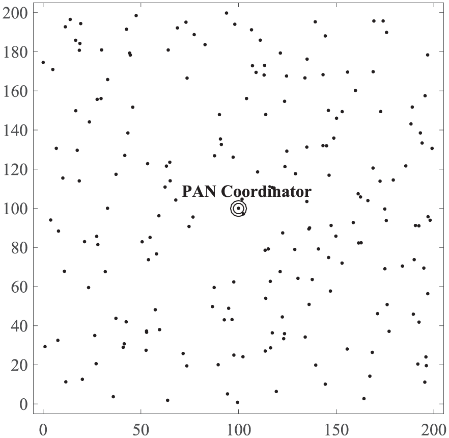
Node deployment using random uniform distribution.

Figure 7.

Node deployment using grid.

Note that these deployment types are suitable for most WSN applications, where the static, grid and random deployments are commonly used. Most of the available simulators also provide different types of deployments. Nevertheless, the main advantage of CT-SIM is the integration between these different deployments and the other cluster-tree functionalities, such as network formation, beacon scheduling, superframe allocation schemes and the multiple communication mechanisms.

Cluster formation

Considering the previously defined scenarios, Figures 8 and 9 illustrate the formation process of a cluster-tree network. For these experiments, we bounded each cluster to a maximum size of eight child nodes (maxChildren parameter). Also, each coordinator (including the PAN coordinator) can select a maximum of three candidate nodes to be CHs (maxCCH parameter). Figure 8 shows a cluster-tree network using a random deployment for the nodes, while Figure 9 shows a cluster-tree network using a grid deployment.

Figure 8.

Random cluster-tree network.

Figure 9.

Grid cluster-tree network.

Table 9 presents some information about the cluster-tree network formation for each deployment. The simulation environment was fully covered using both deployments and all nodes were associated with a particular CH (no orphan nodes).

Table 9.

Information about the cluster-tree network formation.

Information	Random	Grid
Number of clusters	35	43
Average number of nodes (per cluster)	6	5
Maximum depth	6	6

Network addressing

For this set of experiments, we have used hierarchical addressing, in which an addressing block was assigned to each CH based on its number of descendant nodes. For the sake of simplification, Table 10 shows the addressing information of the CHs of depths 0, 1 and 2, considering the random deployment.

Table 10.

List of addressing blocks of the cluster heads, considering the random deployment.

CH	Depth	Network address	Addressing block
0	0	0	[0, 200]
4	1	1	[1, 106]
9	1	107	[107, 145]
27	1	146	[146, 195]
8	2	2	[2, 21]
28	2	22	[22, 53]
35	2	54	[54, 101]
68	2	108	[108, 118]
83	2	119	[119, 126]
103	2	127	[127, 140]
22	2	147	[147, 154]
42	2	155	[155, 185]
86	2	186	[186, 190]

CH: cluster head.

Note that each CH has its own addressing block, in which the first address corresponds to its own network address. It can also be observed that, in these experiments, CHs do not have available addresses to allow new node associations. The hierarchical addressing allows deterministic routing because each CH decides whether a received packet must be forwarded to the parent CH or to its child nodes based on its addressing block.

Cluster scheduling

In order to illustrate the cluster scheduling, Table 11 shows the final scheduling for the top-down and bottom-up cluster scheduling, considering a random deployment. For the sake of convenience, we defined that the cluster ID corresponds to the CH ID.

Table 11.

Cluster scheduling for the random cluster-tree network experiment.

CH	Depth	Top-down	Bottom-up
0	0	1st	35th
4	1	2nd	34th
9	1	3rd	33th
27	1	4th	32th
8	2	5th	31th
28	2	6th	30th
35	2	7th	29th
68	2	8th	28th
83	2	9th	27th
103	2	10th	26th
22	2	11th	25th
42	2	12th	24th
86	2	13th	23th
…	…	…	…
56	4	32th	4th
92	4	33th	3rd
116	5	34th	2nd
101	5	35th	1st

CH: cluster head.

Note that, in the top-down scheduling, the first selected cluster corresponds to the PAN coordinator’s cluster, followed by clusters of depth 1, and, finally, clusters of depth 2. In the bottom-up scheduling, the deepest clusters are first selected. Then, clusters of upper depth are finally selected. It can be observed that the PAN coordinator’s cluster is the last cluster in the scheduling list.

SD allocation

An important CT-SIM functionality is to provide different superframe duration allocation schemes. To the best of our knowledge, no other simulator or simulation model provides this functionality for general WSNs. We have shown that adequate SD allocation is a crucial issue for several WSN applications.^24,26 In order to illustrate this functionality and for the sake of simplicity, we presented some obtained results through the experiments just for the random environment.

Table 12 shows the obtained results by applying a static superframe allocation scheme. In this allocation scheme, all clusters have the same SO parameter defined by beaconOrder simulation parameter.

Table 12.

Static superframe duration allocation scheme for the random cluster-tree network experiment.

CH	Depth	SO	SD (symbols)
0	0	3	7680
4	1	3	7680
9	1	3	7680
27	1	3	7680
8	2	3	7680
28	2	3	7680
35	2	3	7680
68	2	3	7680
83	2	3	7680
103	2	3	7680
22	2	3	7680
42	2	3	7680
86	2	3	7680

CH: cluster head; SO: Superframe Order; SD: Superframe Duration.

In turn, Table 13 shows the obtained results by applying a proportional superframe allocation scheme. In this allocation scheme, SDs are defined based on the load imposed by descendant nodes (nodes belonging to the branch of the CH). The main idea is to allocate adequate bandwidth for each CH in order to improve the network throughput.

Table 13.

Proportional superframe duration allocation scheme for the random cluster-tree network experiment.

CH	Depth	SO	SD (symbols)
0	0	7	122,880
4	1	6	61,440
9	1	4	15,360
27	1	5	30,720
8	2	3	7680
28	2	4	15,360
35	2	5	30,720
68	2	3	7680
83	2	2	3840
103	2	3	7680
22	2	2	3840
42	2	4	15,360
86	2	1	1920

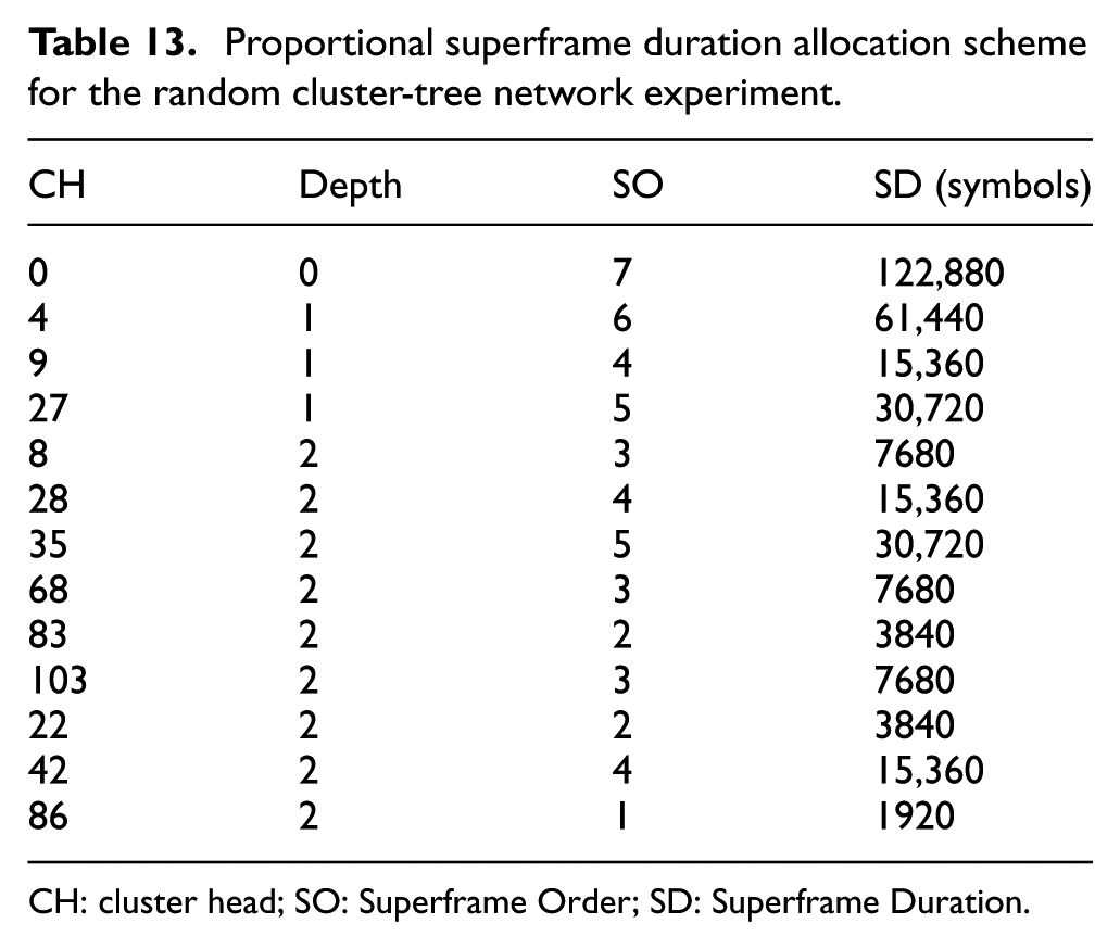
CH: cluster head; SO: Superframe Order; SD: Superframe Duration.

Furthermore, a proportional superframe allocation scheme can also allocate an adequate buffer size for all CHs. The main idea of this allocation scheme is to establish a proper buffer size for each CH based on the message load, allowing to save resources of the nodes. Table 14 shows the size of internal buffers (number of messages) using both the static and proportional superframe duration allocation schemes.

Table 14.

Size of internal buffers of the cluster heads using different superframe duration allocation schemes.

CH	Depth	Static scheme	Proportional scheme
0	0	200	201
4	1	200	106
9	1	200	39
27	1	200	50
8	2	200	20
28	2	200	32
35	2	200	48
68	2	200	11
83	2	200	8
103	2	200	14
22	2	200	8
42	2	200	31
86	2	200	5

CH: cluster head.

Note that for the static allocation scheme, we have defined the size of buffers equal to the number of sensing nodes in the cluster-tree network, without considering any features of the CHs, such as their depths and number of child nodes. In turn, the proportional allocation scheme presents different results by considering the requirements of the network formation process.

The proposed CT-SIM simulation model provides information about the internal buffers of all CHs, such as the average number of messages within the buffers during the active periods of the clusters (via CastaliaResults script). To illustrate this functionality, Figure 10 illustrates the behaviour of the buffers for different depths of the cluster-tree using the top-down cluster scheduling, while Figure 11 illustrates the behaviour of the buffers using the bottom-up scheduling.

Figure 10.

Average number of messages within the buffers of the cluster heads (per depth) using top-down cluster scheduling.

Figure 11.

Average number of messages within the buffers of the cluster heads (per depth) using bottom-up cluster scheduling.

Note that the buffer behaviour is an important metric to analyse the network performance. It can be observed from Figures 10 and 11 that a proportional superframe duration allocation scheme has better performance compared with a static scheme. Besides to save resources, an adequate superframe allocation can avoid the accumulation of messages within the buffers, which could lead to discard messages due to buffer overflows and high delays. For example, Figure 12 illustrates the number of discarded messages due to buffer overflows.

Figure 12.

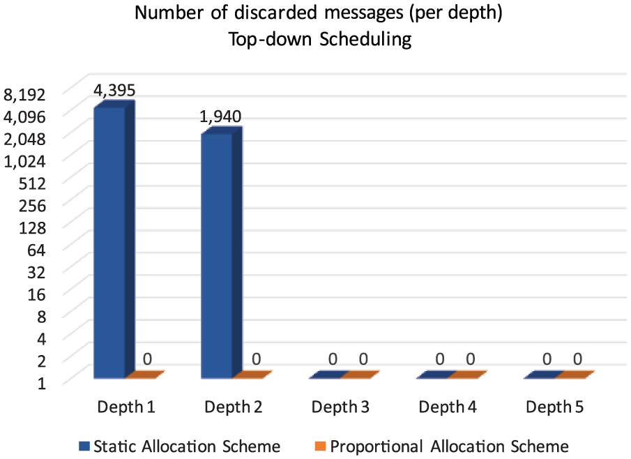
Number of discarded messages within the buffers of the cluster heads (per depth), considering the top-down cluster scheduling.

As it can be seen in Figure 12, the proportional superframe duration allocation scheme may avoid the discard of messages due to buffer overflows, while the static scheme has a high number of discarded messages within the buffers, increasing the message loss rate and the end-to-end delays. This behaviour may be unsuitable for a large number of WSN applications. Therefore, it is important that a simulation model provides mechanisms to evaluate the buffer behaviour of CHs in cluster-tree WSNs.

CP

In order to show the usability of CT-SIM in what concerns the support of different communication traffics, we have performed another set of simulations. First, we performed experiments to illustrate the behaviour of monitoring traffic using different numbers of nodes and data rates. Table 15 shows the different scenarios defined for this experiment.

Table 15.

Set of scenarios to show the communication phase.

Scenario	Number of nodes	Environment size
Scenario 1	50 + PAN	100 m × 100 m
Scenario 2	100 + PAN	141 m × 141 m
Scenario 3	150 + PAN	173 m × 173 m
Scenario 4	200 + PAN	200 m × 200 m

PAN: personal area network.

For all scenarios, the PAN coordinator was placed at the central location of the environment, and the remaining sensing nodes were randomly deployed. Note also that as the number of nodes increases, the environment size proportionally increases in order to keep the same node density. The basic idea is to avoid biased assessments due to the collision effect caused by different node densities.

Regarding data rates, we have defined two types of the monitoring traffic: 0.1 pkt/s (periodicity of 10 s) and 0.05 pkt/s (periodicity of 20 s). For each scenario, data rates were equally distributed among the sensing nodes. The PAN coordinator is the unique node that does not generate data traffic. Each node generates 50 messages.

Figure 13 illustrates the average end-to-end delay for the monitoring traffic, considering the static and proportional superframe duration allocation schemes.

Figure 13.

Average end-to-end delay for the monitoring traffic under different number of sensing nodes.

As the number of nodes increases, the average end-to-end delay also increases due to a higher load of messages. However, we can observe that a proportional superframe duration allocation scheme has a better performance because network parameters were adequately defined according to the number of nodes and the message load imposed by them. Instead, a static allocation scheme does not consider the different conditions for the CHs in order to allocate SDs and buffer sizes, and consequently, the communication delays highly increase.

Additionally, aiming to show the usability of the proposed simulation model regarding the source-to-destination traffic, an experiment was carried out using the two available traffic types together. For this, we have defined an environment size of 200 m × 200 m. Again, the PAN coordinator was deployed in central position. In turn, nodes 1 and 2 were defined as the source and destination nodes for the source-to-destination traffic, respectively. These nodes were statically deployed in opposite positions with the PAN coordinator placed in the middle. Regarding the source-to-destination traffic, node 1 generates 1000 packets towards node 2 with data rate of 0.2 pkt/s (periodicity of 5 s). Nodes 1 and 2 do not generate monitoring traffic. Moreover, we randomly deployed 400 sensing nodes, which generate monitoring traffic. In order to set up different communication scenarios, we defined different monitoring traffic data rates: 0.05 pkt/s (periodicity of 20 s), 0.025 pkt/s (periodicity of 40 s), 0.0166 pkt/s (periodicity of 60 s) and 0.0125 pkt/s (periodicity of 80 s).

Figure 14 illustrates this simulation environment and shows the tree path that supports the cluster-tree communication from node 1 to node 2 (source-to-destination traffic).

Figure 14.

Tree routing for the source-to-destination traffic.

Figure 15 shows the average end-to-end delay for the monitoring and source-to-destination traffics. Note that as the monitoring traffic rate increases, the average end-to-end delay also increases. In fact, increasing the data rate for the monitoring traffic, the number of packets waiting to be transferred in the MAC buffers also increases, inducing higher delays for the packets. Also, there is a large number of nodes trying to contend for the wireless channel. Note also that the source-to-destination traffic keeps a constant end-to-end delay while the data rate increases until the 1 packet every 40 s for the monitoring traffic. However, using the data periodicity of 20 s for the monitoring traffic, the average end-to-end delays increase for both the monitoring and source-to-destination traffics, which shows that the cluster-tree can be saturated.

Figure 15.

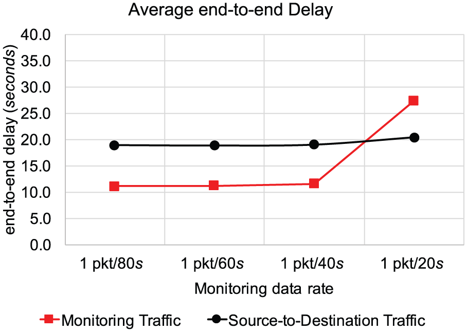
Average delay for the monitoring and source-to-destination traffics.

CT-SIM shortcomings

The major shortcomings of the proposed CT-SIM simulation model are that it still does not implement the IEEE 802.15.4 non-beacon-enabled mode or the GTS scheme. Additionally, only top-down and bottom-up cluster scheduling mechanisms are available. Other state-of-the-art scheduling approaches have still not been implemented, as those proposed by Koubâa et al. ²³ We also intend to improve the SIC module in order to add new performance metrics.

Conclusion and future considerations

In this article, we presented CT-SIM, a set of simulation models proposed for IEEE 80215.4/ZigBee-based cluster-tree WSNs, that was built upon the Castalia simulator. These simulation models allow to build random wide-scale cluster-tree networks, considering their most important mechanisms and issues, such as network formation, addressing, cluster scheduling, SD allocation and direct and indirect data communication mechanisms. We showed through a series of experiments the main features and capabilities of the proposed CT-SIM simulation models.

CT-SIM was designed in a modular way, which allows the configuration of multiple communication environments and network parameters. With this, researchers and developers can design and evaluate new protocols and implementations for wide-scale cluster-tree networks based on the IEEE 802.15.14/ZigBee standards.

As future considerations, we intend to add new functionalities to the proposed simulation model and to implement new communication protocols and approaches for wide-scale cluster-tree networks. Also, we intend to soon make an evaluation version of this simulation model, that will be available for the research community.