Sage Journals: Discover world-class research

Abstract

With the rapid resource requirements of Internet of Things applications, cloud computing technology is regarded as a promising paradigm for resource provision. To improve the efficiency and effectiveness of cloud services, it is essential to improve the resource fairness and achieve energy savings. However, it is still a challenge to schedule the virtual machines in an energy-efficient manner while taking into consideration the resource fairness. In view of this challenge, a fair energy-efficient virtual machine scheduling method for Internet of Things applications is designed in this article. Specifically, energy and fairness are analyzed in a formal way. Then, a virtual machine scheduling method is proposed to achieve the energy efficiency and further improve the resource fairness during the executions of Internet of Things applications. Finally, experimental evaluation demonstrates the validity of our proposed method.

Keywords

Fairness energy Internet of Things applications cloud virtual machine scheduling

Introduction

Internet of Things (IoT), proposed by Prof. Ashton in 1999, has become one of the most popular technologies recently.^1,2 In the past few years, the connotation of IoT has been deployed rapidly, and the applications of IoT continue expanding enormously as well. The IoT has many advanced features, such as intelligent processing, reliable transmission, and full perception. So with the development of IoT technology, IoT applications also increase explosively. IoT applications cover all kinds of areas, such as in U-Home, intelligent transportation, intelligent medical, smart grid, intelligent logistics, environmental protection, intelligent industry, intelligent agriculture, to name a few.^3–5

During the process of IoT applications, cloud computing technology is regarded as a driver for IoT computation enhancement, energy efficient, and service implementation.⁶ Generally, IoT applications can offload the massive computational tasks to the cloud platform to accomplish the large capacity storage and computation.⁷ And the applications are able to obtain the necessary resources of cloud data centers; at the same time, users should pay for the resources. Therefore, the IoT can achieve a scalable computing between mobile client and the cloud.

The energy consumption for the execution of IoT applications is growing at a very high rate while deploying these applications to the cloud platform. And it is considerable that the IoT consists of computational and processing resources, which can be responded by the cloud infrastructure. The exponential growth in the number of IoT applications becomes available in the cloud environment, which leads to massive energy consumption in cloud systems.⁸ What is more, the energy consumption in cloud data center has been a hot topic in Internet Data Center (IDC). So it is necessary to achieve energy savings for IoT applications in cloud environment.

In the cloud environment, the service providers allocate resources to IoT applications in the form of virtual machine (VM). And the resource requirements of IoT applications have many different types, including central processing unit (CPU)-intensive, input/output (I/O)-optimized VM instances, and so on. Meanwhile, to reserve network bandwidth to access the resource pool in cloud is necessary for data processing and storage. In this circumstance, all kinds of resources, such as bandwidth, computation and storage, need to be allocated fairly.⁹ Generally, there are lots of resource requests for IoT applications at the same time, which results in the resource competition during resource management, and such unfair competition may interrupt the services.³ Therefore, resource fairness should be taken into consideration during resource allocation for IoT applications in cloud environment.

However, to the best of our knowledge, few of the works for the VM scheduling have been done for IoT applications in the cloud environment, while taking both energy consumption and resource fairness into consideration. In view of this challenge, a fair energy-efficient VM scheduling method (FEM) for IoT applications is proposed in this article. Our main contributions are threefold. First, fairness analysis and energy consumption analysis in the cloud environment are presented, so that we can investigate the challenge in a formal manner. Second, a corresponding FEM is proposed to achieve the goals of energy savings and fairness enhancement. Finally, comprehensive experiments and simulations are conducted to demonstrate the validity of our proposed method.

The reminder of the article is organized as follows. Section “Resource fairness and energy consumption analysis in cloud environment” provides the fairness and energy consumption analysis in cloud environment. An FEM for IoT applications is proposed in section “An FEM for IoT applications.” Section “Experimental evaluation” presents the experiment results. Finally, section “Related work” discusses related work and section “Conclusion” concludes our work.

Resource fairness and energy consumption analysis in cloud environment

Resource fairness analysis

In cloud data centers, different types of physical machines (PMs) are deployed to provide resources for IoT applications. Denote P = {p₁, p₂, …, p_N} as the PM list running in the data centers, where N is the number of PMs in P. Each PM is equipped with various physical resources, including CPU, memory, bandwidth, and so on. Suppose there are M types of resources contained among the PMs in P, denoted as R = {r₁, r₂, …, r_M}.

The resource fairness for a PM is relevant to the resource utilization for each type of resource. The resource utilization of the PMs can be calculated according to the resource amount and resource usage. Generally, the resource amount and the resource usage can be measured by the number of resource units. Let pr_n,m be the resource in the nth PM p_n with the mth resource type r_m. For pr_n,m, the resource usage is denoted as u_n,m, and the resource amount is denoted as c_n,m.

The submitted IoT applications should rent a definite amount of resources to respond to the application execution. IoT applications contain a large amount of tasks. Suppose there are W tasks contained in the applications, denoted as T = {t₁, t₂, …, t_W}. All the tasks in T have personalized resource requests for different types of resources, including CPU, memory, and so on.

Definition 1 (resource request)

For t_w (1 ≤ w ≤ W), the resource request, denoted as q_w = {q_w,1, q_w,2, …, q_w,M}, consists of the specific resource amount of each type of resource.

In q_w, q_w,m represents the requested resource amount of the mth (1 ≤ m ≤ M) resource type for task t_w. As the resources in the cloud environment are provisioned in the form of VMs, the resource requests from IoT applications need to be presented by the VMs with specific resource amounts. The VMs allocated for the tasks in T are denoted as V = {v₁, v₂, …, V_W}, where v_w (1 ≤ w ≤ W) represents the VM for task t_w.

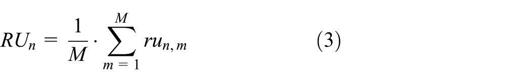
The resource utilization of the PM p_n for resource type r_m, denoted as ru_n,m, is calculated by

r u_{n, m} = \frac{\sum_{w = 1}^{W} I_{w}^{n} \cdot q_{w, m}}{c_{n, m}}

(1)

where $I_{w}^{n}$ is a binary variable to judge whether v_w is placed on p_n, which is calculated by

I_{w}^{n} = {\begin{matrix} 1, if v_{w} is placed on p_{n} \\ 0, otherwise \end{matrix}

(2)

Then the resource utilization of p_n for all the resources is calculated by

R U_{n} = \frac{1}{M} \cdot \sum_{m = 1}^{M} r u_{n, m}

(3)

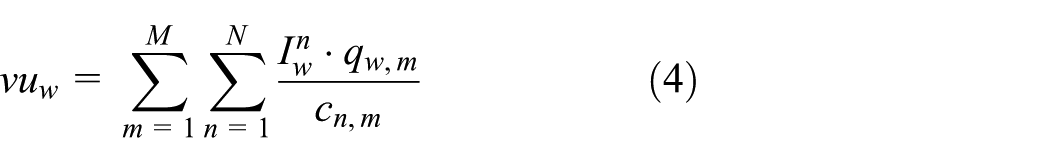
The resource fairness is closely related to the resource utilization for all types of resources and the resource utilization of each VM. The resource utilization of v_w is relevant to the total resource usage of the VM, denoted as vu_w, which is calculated by

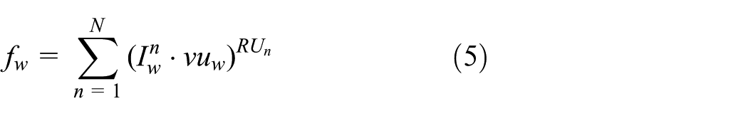
v u_{w} = \sum_{m = 1}^{M} \sum_{n = 1}^{N} \frac{I_{w}^{n} \cdot q_{w, m}}{c_{n, m}}

(4)

Based on the fairness computation analysis in Ghodsi et al.¹⁰ and Wang et al.,¹¹ the resource fairness in PM v_w is calculated by

f_{w} = \sum_{n = 1}^{N} {(I_{w}^{n} \cdot v u_{w})}^{R U_{n}}

(5)

Energy consumption analysis

For IoT applications submitted to the cloud platforms, they need a large amount of energy consumption to guarantee execution efficiency. In the large-scale data centers, the energy consumption by network devices, security devices, cooling systems, and so on has been considered to be more. As IoT applications consume a large number of physical resources, including computation, storage, and so on, we mainly focus on the energy consumption due to the execution of IoT applications. Efficient VM scheduling strategies can contribute to reduce the energy consumption in cloud data centers, since the energy consumed by the cooling system and other devices depends on the energy consumption in the servers. Thus, in this article, we try to achieve energy savings during the execution of IoT applications. In the cloud data centers, the energy consumption mainly refers to three aspects, including the PM base energy consumption, the energy consumption by the running VMs, and the energy consumption by VM communications.^12,13 The unused resources on the PM also consume a certain amount of energy, but it is not the dominant part of the energy consumption. Thus, in our energy consumption model, the PM base energy consumption and the VM energy consumption are taken into consideration.

The PMs in the data centers have three modes, that is, active mode, idle mode, and sleep mode. The PM is in the active mode when it is employed for application execution. During the lifetime of IoT applications, the PMs should consume the base energy. The lifetime of a PM is determined by the occupation time of the VMs deployed on it. For p_n, the lifetime, denoted as l_n, is calculated by

l_{n} = {max}_{w = 1}^{W} {I_{w}^{n} \cdot λ_{w}}

(6)

where λ_w is the occupation time of v_w.

Then the base energy consumption for all the PMs is calculated by

BE = \sum_{n = 1}^{N} α_{n} \cdot l_{n}

(7)

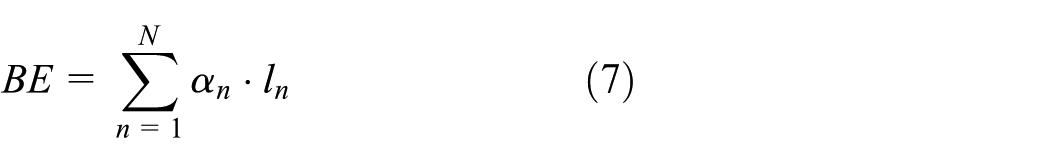
where α_n is the base energy consumption rate of p_n, that is, the energy consumption of p_n per unit time.

The energy consumption by the running VMs is denoted as VE, which is calculated by

VE = \sum_{w = 1}^{W} β_{w} \cdot λ_{w}

(8)

where β_w is the energy consumption rate for v_w in the active mode.

The VMs in the idle mode also consume a certain amount of energy, denoted as IE, which is calculated by

IE = \sum_{n = 1}^{N} \sum_{w = 1}^{W} γ_{w} \cdot (l_{n} - λ_{w})

(9)

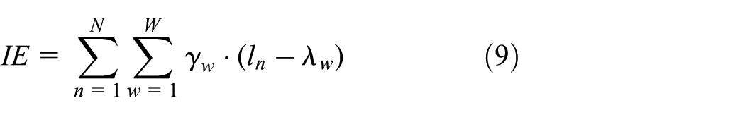
where β_m is the energy consumption rate of s_m in idle mode.

In addition, the energy consumption due to data transmission among VMs during task execution also should be taken into consideration. The energy consumption for the VM communications, denoted as TE, is calculated by

TE = \sum_{w = 1}^{W} \sum_{w' = 1}^{W} \frac{D_{w, w'}}{θ_{w, w'}} \cdot δ_{w, w'}

(10)

where D_w,w′ is the total data size transferred from v_w to v_w_′, θ_w,w_′ is the bandwidth between v_w and v_w_′, and δ_w_′ is the energy consumption rate for data transmission between v_w and v_w_′.

After the above analysis, the total energy consumption for IoT application executions is calculated by

E = BE + VE + IE + TE

(11)

An FEM for IoT applications

PM resource monitoring and idle space detection

To facilitate VM scheduling for IoT applications, the task requests of IoT applications are quantified by each type of resources in section “Resource fairness analysis.” To schedule VMs in an energy-efficient and fair manner, the unused resources should be identified. Therefore, it is essential to monitor the resource usage for each type of resources. In this article, in order to monitor the usage for each type of resource in the PMs and detect idle resources further, a resource occupation table is defined as follows.

Definition 2 (resource occupation table)

The resource occupation table ROT_n (1 ≤ n ≤ N) is used to keep a track of the VM occupation records in the PM p_n, which are generated when p_n is leveraged to respond to the resource requests for VM placement.

Generally, several VMs could be placed on the same PM, thus there are a set of VM occupation records contained in ROT_n. Let z_n be the number of VM occupation records in ROT_n. For the ith (1 ≤ i ≤ z_n) VM occupation record rot_n,i, it is a three-tuple, which is defined by rot_n,i = {rv_n,i, st_n,i, dt_n,i}, where rv_n,i is the VM that is placed on p_n and st_n,I, and dt_n,i are the service start time and duration time for the VM on p_n, respectively.

The resource occupation table of a PM is dynamically updated under two situations. On one hand, when a new VM is mapped on the PM, the PM will provide all the resources for the VM to support the task execution deployed on the VM, and the resource occupation is updated. On the other hand, the resource occupation table also needs to be updated when the VMs on the PM migrate to another PM, since the duration time of the VM is changed during VM running.

Algorithm 1 specifies the process of resource occupation table updating. In this algorithm, the new arrival VM will generate a new VM occupation record after the VM is mapped to this PM (Lines 1–4). Then if the VM on p_n migrates to another PM during execution, the relevant occupation record is identified and updated (Lines 5–16).

Algorithm 1 Resource occupation table updating.
Input: The resource allocation table ROT_n, the task request tag TAG, the VM v need to be processed, and the update time t
Output: The updated resource occupation table ROT_n
1: if TAG == VMInthen
2: a = z_n + 1
3: Generate a record rot_n,a for v
4: Add rot_i,a to ROT_n
5: else if TAG == VMOutthen
6: flag = 1
7: i = z_n
8: while flag == 1 do
9: if rv _n,i == vthen
10: dt_n,i = t − st_n,i
11: flag = 0
12: else i = i − 1
13: end if
14: end while
15: end if
16: end if

Through statistics and analysis of the resource allocation table, the amount of each type of idle resources can be detected at any time. Let ia_n = {ia_n,1, ia_n,2, …, ia_n,m} be the resource set to record M types of resources, where ia_n,m (1 ≤ m ≤ M) is the idle amount of the resource with resource type r_m.

Algorithm 2 specifies the process of idle resource detection. In this algorithm, to get the idle amount of each type of resource, we should traverse all the VM occupation records (Line 1). Then according to the VM and time attributes in these records, the finish time of each type of resource can be calculated (Lines 2 and 3). Furthermore, the occupied amount for all resources can be counted (Lines 4–9). After these steps, the final idle resource amount can be counted (Lines 11–13).

Algorithm 2 Idle resource detection.
Input: The resource occupation table RoT_n and detection time t
Output: The idle amount of each type of resource ia_n
1: for i = 1 to z_ndo
2: Get v from rot_n,i
3: ft = st_n,i + dt_n,i
4: if ft > tthen
5: for m = 1 to Mdo
6: Get the occupied amount o_n,m for resource type r_m
7: x_n,m = x_n,m + o_n,m
8: end for
9: end if
10: end for
11: for m = 1 to Mdo
12: ia_n,m = c_n,m − x_n,m
13: end for

PM identification and classification

Each PM has a dominant resource. To better fit the resource requirements of the tasks in IoT applications, the PMs should be classified according to the dominant resource.

A cloud vendor provides a variety of VMs with different configurations for cloud renters. For example, Amazon EC2 provides various VM instance types to accommodate the demand performance of cloud renters, including CPU-optimized instances, high I/O instances, and so on.¹⁴ Generally, if the dominant resource of a PM is CPU, this PM is employed to respond to the CPU-optimized VMs.

As there are M types of resources in the cloud data centers and each PM has a dominant resource, the PMs in P could be classified into M types. Let rs_m be the PM collection with mth dominant resource. However, the PMs that have spare dominant resources can be selected for VM scheduling. In this article, a threshold ρ is employed to judge whether the PM is overload. To avoid PM overload, the PMs whose resource utilization are less than ρ are identified. Based on the PM resource monitoring and idle resource detection in section “PM resource monitoring and idle space detection,” the usage amount and the idle amount of each type of resource can be detected dynamically. The usage amount for each type is necessary to calculate the resource utilization of PM by equation (3). Then, according to the resource type and the resource utilization, the PMs are classified and identified to the relevant PM collection.

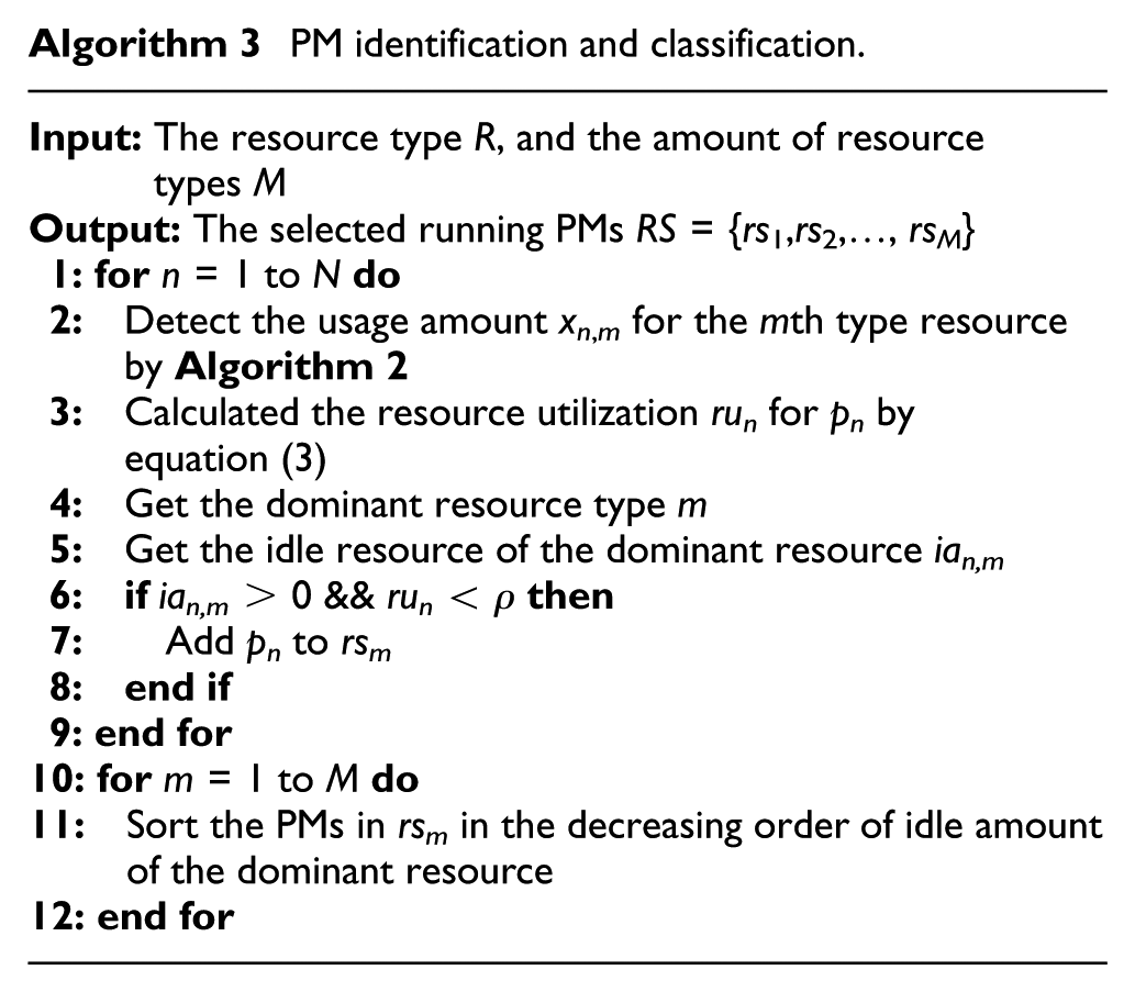
Algorithm 3 specifies the process of PM identification and classification. In this algorithm, we traverse all the PMs in P (Line 1), and the usage amount for each type of resource is detected by Algorithm 2 (Line 2). Based on the usage values for all types of resources, the resource utilization of the PM is calculated (Line 3). For further PM classification, the dominant resource type of p_n should be identified (Line 4), and the idle resource of the dominant resource should also be detected (Line 5). Then the PM with enough spare dominant resources and whose resource utilization is not over the threshold ρ is identified and added to the relevant PM set (Lines 6–8). As the PMs with more idle resources will be chosen for VM scheduling, the PMs in the classified PM sets should be sort in the decreasing order of idle amount of the dominant resource (Lines 10–12).

Algorithm 3 PM identification and classification.
Input: The resource type R, and the amount of resource types M
Output: The selected running PMs RS = {rs₁,rs₂,…, rs_M}
1: for n = 1 to Ndo
2: Detect the usage amount x_n,m for the mth type resource by Algorithm 2
3: Calculated the resource utilization ru_n for p_n by equation (3)
4: Get the dominant resource type m
5: Get the idle resource of the dominant resource ia_n,m
6: if ia_n,m > 0 && ru_n < ρthen
7: Add p_n to rs_m
8: end if
9: end for
10: for m = 1 to Mdo
11: Sort the PMs in rs_m in the decreasing order of idle amount of the dominant resource
12: end for

Energy-efficient VM scheduling

VM live migration is one of the most essential technologies for cloud computing, which supports running VM mapped from one PM to another, and it avoids interrupting the running application.¹⁵ For the running VMs in V, they can benefit from the VM live migration technology. By leveraging this technology, the VMs on the PMs with low-resource utilization will be moved to the PMs with high-resource utilization.

The resource requests of the tasks in IoT applications have various dominant resources. Thus, the VMs, rented for hosting the tasks, should be placed on the PMs with the same dominant resources. For example, a CPU-intensive VM should be mapped to a CPU-intensive PM for running. According to the specific analysis of PM identification and classification in section “PM identification and classification,” the PMs are classified by the resource type.

For the VMs running in the mth PM set rs_m, the PMs are sorted in the decreasing order of the idle amount of the dominant resources. When all the VMs on a PM are all migrated to the other PMs, this PM would be empty, and it could be set to the sleep mode to achieve energy savings. The PMs with lowest resource utilization will be handled first. If all the VMs on this PM can be migrated to the PMs in rs_m with higher PMs, a scheduling policy is generated.

Definition 3 (scheduling policy on PM)

A scheduling policy on a PM consists of a set of VM migration strategies, denoted as S = {s₁, s₂, …, s_K}, where K is the number of VM migrations.

Definition 4 (VM migration strategy)

For the kth (1 ≤ k ≤ K) VM migration strategy in S, it is a four-tuple, denoted as s_k = {mv_k, op_k, dp_k, mt_k}, where mv_k is the migrated VM, op_k is the origin PM the VM deployed, dp_k is the destination PM where the VM migrated, and mt_k is the migration time.

The PMs are handled according to the PM order in rs_m. After each turn of VM scheduling policy generation, the resource utilization of all the PMs in rs_m is updated. The PMs with no spare dominant resources are removed from rs_m. And according to the generated scheduling policies on all PMs, the scheduling policy for each VM in V can be updated. Let X = {x₁, x₂, …, x_w} be the VM scheduling policies for all VMs in V.

Definition 5 (VM scheduling policy)

For the wth (1 ≤ w ≤ W) VM scheduling policy x_w in X, it is a three-tuple, denoted as x_w = {sp_w, dp_w, ot_w}, where sp_w, dp_w, and ot_w represent the migration start time, the original PM, and the destination PM, respectively.

Algorithm 4 specifies the process of energy-efficient VM scheduling (EVS). In this algorithm, the PMs are identified and classified according to the resource types and the idle amount of the dominant resources by Algorithm 2 (Line 1). Then we traverse the obtained PM sets and handle the VMs for each PM set (Line 2). All the available VM scheduling policies are generated for each PM set (Lines 3–24).

Algorithm 4 Energy-efficient VM scheduling.
Input: The PM set P, the VM set V
Output: The VM migration policy
1: Algorithm 2: PM identification and classification.
2: for m = 1 to Mdo
3: Get the number of PMs in rs_m, denoted as np
4: for i = 1 to npdo
5: Get the number of VMs on the PM, denoted as nv
6: q = np
7: for i = 1 to nvdo
8: flag = 1
9: while flag == 1 do
10: if qth PM can host the ith VM then
11: Generate the VM migration strategy
12: flag = 0
13: else q = q − 1
14: end if
15: end while
16: end for
17: if all the VMs in the PM can be migrated away then
18: Generate scheduling policy for the VMs
19: Update the relevant VM scheduling policies
20: Update the resource occupation table
21: Remove the PM from rs_m
22: else Remove the VM migration strategies
23: end if
24: end for
25: end for

Fairness-aware VM scheduling

After the EVS, the VMs are placed using least PMs with the same dominant resources. However, the resources in these PMs may not be fairly employed, since the main resources consumed are the dominant resources. To use the resource in a fair manner, fairness-aware VM scheduling is necessary.

To improve the resource fairness in the cloud environment for IoT applications, the part of VMs running on the PMs with the same dominant resource should be migrated to the other PMs with the other dominant resources. For example, if there is a PM with dominant resource CPU, and to execute the computing tasks in IoT applications, there are several CPU-optimized VMs running on it, and few of the I/O resources in this PM have been used. In order to improve the overall fairness in the whole data centers, the I/O-optimized VMs could be migrated to this PM. After fairness-aware scheduling, part of the running PMs, may be empty, and they can be set to sleeping mode to achieve further energy savings.

In section “PM identification and classification,” the running PMs are classified by the dominant resources. Full utilization of the idle resources on the PMs contributes to improving the fairness. Thus, the resource utilization for each type of resource should be obtained first. Then we get the resource type with the minimum resource utilization. For the PM sets in RS, the PM set whose dominant resources are with this obtained resource type is identified. The PMs in the identified PM set are sort in the increasing order of the fairness values, which can be calculated by formula (5). The PM with lower fairness values will have a higher priority to be processed, and the VMs on this PM are considered to be migrated away. All the VMs are sort in the increasing order of the amount of the dominant resources. The VMs with fewer resource requests will be handled first. After VM migration, the corresponding VM scheduling policies, the resource occupation table, and the PM mode are updated accordingly.

Algorithm 5 specifies the process of fairness-aware VM scheduling. In this algorithm, we traverse all the PM sets after processing by Algorithm 4 (Line 1). Then the numbers of PMs in each PM set are obtained for fairness analysis. Each PM in the PM set will be analyzed, especially on the resource utilization values for each type of resource, the resource type with minimum resource utilization value, and the PM set with the obtained resource type (Lines 4–6). Then the identified PM set is handled by the fairness values (Lines 7–10). Furthermore, the VMs are scheduled to migrate to the identified PMs with idle space (Lines 11–26).

Algorithm 5 Fairness-aware VM scheduling.
Input: The PM set P, the VM set V
Output: The VM scheduling policies
1: for m = 1 to Mdo
2: Get the number of PMs in rs_m, denoted as np
3: for i = 1 to npdo
4: Calculate the resource utilization for each type of resource
5: Get the resource type m_′ with minimum resource utilization
6: Get the PM set rs_m′ in RS with the obtained resource type
7: for each PM in rs_m′do
8: Get the resource utilization by equation (4)
9: Get the fairness values by equation (5)
10: end for
11: Sort the PMs in rs_m′ in the increasing order of fairness values
12: Get the number of PMs in rs_m′, denoted as np′
13: j = 0, flag = 1
14: while flag == 1 do
15: Sort the VMs in the increasing order of dominant resource
16: for each VM in rs_m′,jdo
17: if the VM can be migrated to rs_m,ithen
18: Update the resource occupation table
19: Update the VM scheduling policy
20: j = j + 1
21: else flag = 0
22: end if
23: end for
24: end while
25: end for
26: end for

Experimental evaluation

In this section, a number of simulations and experiments are conducted to evaluate the performance of our proposed FEM. The simulation framework CloudSim is employed to model the cloud infrastructure. For comparison analysis, the running state without migration is treated as a benchmark. Besides, the EVS method presented in section “Energy-efficient VM scheduling” is also employed for comparison analysis.

Experimental context

In the experiments, four types (type 1–type 4) of PMs are applied to construct the cloud simulation infrastructure, that is, type 1: HP ProLiant ML110 G4 (Intel Xeon 3040, dual-processor clocked at 1860 MHz, 4 GB of RAM), type 2: HP ProLiant ML110 G5 (Intel Xeon 3075, dual-processor clocked at 2660 MHz, 4 GB of RAM), type 3: HP ProLiant BL460c G6 (Intel Xeon 5630, quad-processor clocked at 2530 MHz, 8 GB of RAM), and type 4: HP ProLiant SL390s (G7 Intel Xeon 5649, hexa-processor clocked at 3060 MHz, 16 GB of RAM).^12,13

The specification of these four types of PMs is listed in Table 1. In the simulated cloud environment, 1000 PMs are created and the amount of each type of the PMs is 250. Based on Beloglazov and Buyya,¹⁶ the power consumption of type 1 and type 2 PMs is set to 86 and 93.7 W, separately. And based on the HP operation documents, the peak power consumption of type 3 and type 4 PMs for each processor is set to 80 and 95 W, separately.^12,13 As the PM consumes nearly 60% of the power, the power consumption of type 3 and type 4 PMs is set to 192 and 342 W in this article, separately.^12,13,17,18

Table 1.

Parameter settings.

Parameter item	Domain
Number of running PMs	{500, 1000, 1500, 2000, 2500, 3000}
Number of running VMs on each PM	[1, 3]
Number of dominant resources for four types of PMs	{6, 8, 16, 32}
Number of the non-dominant resources	[1, 5]
Duration time of each VM	[0.5, 3]

PM: physical machine; VM: virtual machine.

There are five basic parameters in our experiment. For each parameter, its value domain is specified in Table 1. More specifically, six datasets of IoT applications with different scales are generated for our simulation. The dataset contains a number of VM running records for the running PMs, and the PM amounts for these six datasets in our experiments are set to 500, 1000, 1500, 2000, 2500, and 3000, respectively. Each data record in these datasets is described as an eight-tuple. An instance of a data record is (10, 7, 3, 2, 1, 0, 0, 0.5). And it means that the 10th task from IoT applications is running on the third VM deployed on the seventh server. This task requires the resources on the PM; “2” is the amount of the dominant resource. The resource requirements for the non-dominant resources are 1, 0, and 0, respectively. Besides, these resources constitute the VM, which needs to run 0.5 h on this PM.

Performance evaluation

In this section, performance evaluations on energy consumption and fairness are discussed to demonstrate the validity of our proposed method.

Performance evaluation w.r.t. energy consumption

As the running PMs need to consume the base energy, the number of running PMs is closely relevant to the energy consumption. Figure 1 shows the comparison of the number of PMs after scheduling using six different scales of datasets. As illustrated in Figure 1, we can find that after VM scheduling by leveraging the VM migration technique, FEM employs fewer PMs than benchmark and EVS.

Figure 1.

Comparison of number of PMs after scheduling by benchmark, EVS, and FEM.

Based on the energy consumption analysis in section “Energy consumption analysis,” the energy consumption after IoT application executions can be obtained. Figure 2 shows the comparison of total energy consumption after scheduling by benchmark, EVS, and FEM. As shown in Figure 2, we can find that FEM can achieve more energy savings, compared with benchmark and EVS. For example, when the number of servers is 3000, the energy consumption caused by FEM is less than 1 GW h, but benchmark and EVS consume more than 1 GW h.

Figure 2.

Comparison of total energy consumption after scheduling by benchmark, EVS, and FEM.

There are four types of PMs employed in our evaluations, and thus four types of dominant resources are presented in the experiment. For more specified analysis of energy consumption, the comparison analysis for different types of PMs should be presented. Figure 3(a)–(d) shows the comparison of energy consumption for different types of PMs by benchmark, EVS, and FEM. From these figures, we can find that FEM can save more energy than benchmark and EVS. For example, in Figure 3(a), when the type of dominant resource is four, for different scales of datasets, FEM saves more energy than benchmark and EVS.

Figure 3.

Comparison of energy consumption for different types of PMs by benchmark, EVS, and FEM: (a) type of dominant resource = 1, (b) type of dominant resource = 2, (c) type of dominant resource = 3, and (d) type of dominant resource = 4.

Performance evaluation w.r.t. resource fairness

The resource fairness is decided by the utilization of the dominant resources and the PM average utilization. We investigate these values by benchmark, EVS, and FEM using six different datasets.

Figure 4 shows the comparison of average utilization of the dominant resource by benchmark, EVS, and FEM. As illustrated in Figure 4, FEM can achieve higher utilization of the dominant resources than benchmark and EVS. Although sometimes EVS can get utilization values similar to FEM, overall FEM is better than EVS.

Figure 4.

Comparison of average utilization of dominant resource by benchmark, EVS, and FEM.

Figure 5 shows the comparison of average PM resource utilization by benchmark, EVS, and FEM. As illustrated in Figure 4, FEM can achieve higher PM resource utilization than benchmark and EVS. For example, when the number of servers is 500, the utilization achieved by FEM is nearly 70%, while the utilization values obtained by EVS and benchmark are nearly 30% and 10%, respectively. We can deduce that more non-dominant resources are spared on the PMs when using EVS, compared with FEM.

Figure 5.

Comparison of average PM resource utilization by benchmark, EVS, and FEM.

Figure 6 shows the comparison of average fairness value after scheduling by benchmark, EVS, and FEM. From Figure 6, we can find that FEM can achieve higher fairness values compared with EVS and benchmark. For example, when the number of servers is 2000, the fairness value by FEM is about 3, but the fairness generated by EVS and benchmark (about 1.5 and 1, respectively) are much smaller than this value.

Figure 6.

Comparison of average fairness value after scheduling by benchmark, EVS, and FEM.

Table 2 shows the improvements of resource fairness with EVS and FEM compared to benchmark. It is intuitive from Figure 6 and Table 2 that our proposed FEM can obtain the best fairness value.

Table 2.

Improvements of resource fairness with EVS and FEM compared to benchmark.

Scheduling method	Number of servers
Scheduling method	500	1000	1500	2000	2500	3000
EVS (%)	33.11	30.67	37.43	43.58	41.09	45.07
FEM (%)	54.59	83.02	93.31	107.42	115.13	130.61

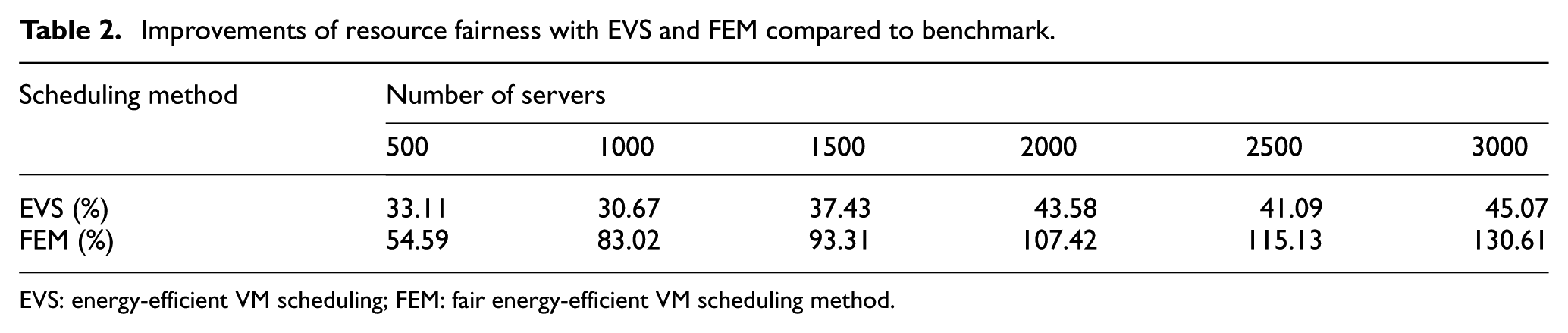
EVS: energy-efficient VM scheduling; FEM: fair energy-efficient VM scheduling method.

Related work

IoT applications have great development in all kinds of circumstances, and the capacity of computing and storage is limited for itself. So it has been deployed to the cloud platform to achieve the demand of the applications. They have been fully investigated in Wang et al.,⁸ Tomita and Kuribayashi,⁹ Khan et al.,³ and Ghodsi et al.,¹⁰ to name a few.

Wang et al.⁸ proposed an architecture that automates allocation and monitoring, and redistributes both cloud and cellular network resources to achieve economies of scale and automation in management of IoT applications. In order to deploy the smart city applications, Kaur et al.¹⁹ addressed the convergent domain of cloud computing and IoT. Namal et al.²⁰ came up with an autonomic trust management framework in cloud-based and highly dynamic IoT applications to evaluate the level of trust.

The current researches mainly focus on realizing efficient resource allocation in IoT environments. Angelakis et al.²¹ devised two algorithms to get the approximate optimal solution for an IoT device equipped with flexible services. Kim et al.²² proposed a service resource allocation approach to minimize data transmissions between mobile devices and effectively deal with the constraints in IoT environments. Renner et al.²³ formulated a container-based resource allocation scheme for the IoT to increase the utilization and reduce the amount of generated network traffic.

What is more, there has been much work dealing with the fair resource allocation in cloud environment. Wang and colleagues¹³ designed a multi-resource allocation mechanism, which provides many kinds of highly desirable properties. With this allocation mechanism, the authors achieved multi-resource fair allocation in heterogeneous cloud computing systems. Tang et al.²⁴ proposed a novel fair resource allocation mechanism for data-intensive computing in the cloud, and it successfully overcame the challenge of “big data.” Generally speaking, fairness and energy consumption are of importance to generate IoT applications on cloud platform. Thus, this article proposed the fair energy-efficient resource allocation for IoT applications in cloud environment.

Conclusion

In this article, we propose an FEM for IoT applications in cloud environment, which is based on VM migration technology. It aims to achieve the goal of energy savings and fairness improvement. We analyze the energy consumption and the resource fairness in the cloud environment to formalize our problem. And a corresponding VM scheduling method is designed to solve this problem. The experimental results demonstrate the validity of our method.

Footnotes

Academic Editor: Xuyun Zhang

Declaration of conflicting interests

The author(s) declared no potential conflicts of interest with respect to the research, authorship, and/or publication of this article.

Funding

The author(s) disclosed receipt of the following financial support for the research, authorship, and/or publication of this article: This research was partially supported by the National Science Foundation of China under grant nos 41275116 and 61672290. Besides, it has also been supported by the project of “Six Talent Peaks Project in Jiangsu Province” under grant no. XYDXXJS-040.

References

Zhong

Zhu

Huang

. Study on the IOT architecture and gateway technology. In: 14th international symposium on distributed computing and applications for business engineering and science (DCABES), Guiyang, China, 18–24 August 2015, pp.196–199. New York: IEEE.

Gubbi

Buyya

Marusic

. Internet of Things (IoT): a vision, architectural elements, and future directions. Future Generat Comput Syst 2013; 29: 1645–1660.

Khan

Zaheer

. Future internet: the internet of things architecture, possible applications and key challenges. In: 10th international conference on frontiers of information technology, Islamabad, Pakistan, 17–19 December 2012, pp.257–260. New York: IEEE.

Nastic

Sehic

Vögler

. PatRICIA—a novel programming model for IoT applications on cloud platforms. In: IEEE 6th international conference on service-oriented computing and applications, Koloa, HI, 16–18 December 2013, pp.53–60. New York: IEEE.

Gyrard

Datta

Bonnet

. Cross-domain internet of things application development: M3 framework and evaluation. In: 3rd international conference on future internet of things and cloud, Rome, 24–26 August 2015, pp.9–16. New York: IEEE.

Abdelwahab

Hamdaoui

Guizani

. Replisom: disciplined tiny memory replication for massive IoT devices in LTE edge cloud. IEEE Inter Things J 2016; 3: 327–338.

Bonomi

Milito

Zhu

. Fog computing and its role in the internet of things. In: Proceedings of the first edition of the MCC workshop on mobile cloud computing, Helsinki, 17 August 2012, pp.13–16. New York: ACM.

Wang

Liang

Multi-resource fair allocation in heterogeneous cloud computing systems. IEEE T Parall Distr 2015; 26(10): 2822–2835.

Tomita

Kuribayashi

. Congestion control method with fair resource allocation for cloud computing environments. In: IEEE pacific rim conference on communications, computers and signal processing (PacRim), Victoria, BC, Canada, 23–26 August 2011, pp.1–6. New York: IEEE.

10.

Ghodsi

Zaharia

Shenker

. Choosy: max-min fair sharing for datacenter jobs with constraints. In: Proceedings of the 8th ACM European conference on computer systems, Prague, 15–17 April 2013, pp.365–378. New York: ACM.

11.

Wang

Liang

Dominant resource fairness in cloud computing systems with heterogeneous servers. In: IEEE conference on computer communications, Toronto, ON, Canada, 27 April–2 May 2014, pp.583–591. New York: IEEE.

12.

Dou

Zhang

. EnReal: an energy-aware resource allocation method for scientific workflow executions in cloud environment. IEEE Trans Cloud Comput 2016; 4(2): 166–179.

13.

Wang

. A virtual machine scheduling method for trade-offs between energy and performance in cloud environment. In: International conference on advanced cloud and big data, Chengdu, China, 13–16 August 2016, pp.246–251. New York: IEEE.

14.

Amazon EC2 instances, https://aws.amazon.com/ec2/instance-types/.

15.

Zheng

TSE

Sripanidkulchai

. Pacer: a progress management system for live virtual machine migration in cloud computing. IEEE T Netw Serv Manage 2013; 10(4): 369–382.

16.

Beloglazov

Buyya

Optimal online deterministic algorithms and adaptive heuristics for energy and performance efficient dynamic consolidation of virtual machines in cloud data centers. Concurr Comp: Pract E 2012; 24(13): 1397–1420.

17.

Meisner

Gold

Wenisch

TF.

PowerNap: eliminating server idle power. Comput Architect News 2009; 37(1): 205–216.

18.

Karapantelakis

Liang

Wang . DevOps for IoT applications using cellular networks and cloud. In: IEEE 4th international conference on future internet of things and cloud (FiCloud), Vienna, 22–24 August 2016, pp.340–347. New York: IEEE.

19.

Kaur

Maheshwari

Building smart cities applications using IoT and cloud-based architectures. In: IEEE conference on industrial informatics and computer systems (CIICS), Sharjah, 13–15 March 2016, pp.1–5. New York: IEEE.

20.

Namal

Gamaarachchi

MyoungLee

. Autonomic trust management in cloud-based and highly dynamic IoT applications. In: ITU kaleidoscope: trust in the information society (K-2015), Barcelona, 9–11 December 2015, pp.1–8. New York: IEEE.

21.

Angelakis

Avgouleas

Pappas

. Allocation of heterogeneous resources of an IoT device to flexible services. IEEE Inter Things J 2015; 3(5): 691–700.

22.

Kim

I-Y

. An efficient resource allocation approach based on a genetic algorithm for composite services in IoT environments. In: IEEE international conference on web services (ICWS), New York, 27 June–2 July 2015, pp.543–550. New York: IEEE.

23.

Renner

Meldau

Kliem

. Towards container-based resource management for the internet of things. In: International conference on software networking (ICSN), Jeju Island, South Korea, 23–26 May 2016, pp.1–5. New York: IEEE.

24.

Tang

Lee

Fair resource allocation for data-intensive computing in the cloud. IEEE Trans Serv Comput 2016; (99). DOI: 10.1109/TSC.2016.2531698.

Fair energy-efficient virtual machine scheduling for Internet of Things applications in cloud environment

Abstract

Keywords

Introduction

Resource fairness and energy consumption analysis in cloud environment

Resource fairness analysis

Definition 1 (resource request)

Energy consumption analysis

An FEM for IoT applications

PM resource monitoring and idle space detection

Definition 2 (resource occupation table)

PM identification and classification

Energy-efficient VM scheduling

Definition 3 (scheduling policy on PM)

Definition 4 (VM migration strategy)

Definition 5 (VM scheduling policy)

Fairness-aware VM scheduling

Experimental evaluation

Experimental context

Performance evaluation

Performance evaluation w.r.t. energy consumption

Performance evaluation w.r.t. resource fairness

Related work

Conclusion

Footnotes

Declaration of conflicting interests

Funding

References