Measurement of the electric energy storage capacity in solar thermoelectric generators’ energy harvesting modules

Abstract

Reducing energy consumption is mandatory in self-powered sensor nodes of wireless sensor networks that obtain all their energy from the environment. In this direction, one first step to optimize the network is to accurately measure the total energy harvested, which will determine the power available for sensor consumption. We present here a technique based on an embedded circuit with an ultra-low-power microcontroller to accurately measure the efficiency of flat-panel solar thermoelectric generators operating with environmental temperature gradients. Experimental tests showed that when a voltage of 180 mV (best case in an environmental flat-panel solar thermoelectric generators) is applied to the input of the DC–DC converter, the proposed technique eliminates a measurement error of 33% when compared with the conventional single supercapacitor strategy.

Introduction

Energy harvesting systems based on flat-panel solar thermoelectric generators (STEGs) are an excellent green and sustainable alternative for powering environmental sensor networks. The monitoring or detection of environmental parameters for precision agriculture,^1–3 monitoring of water quality in remote water sources, ⁴ pollution in remote locations, ⁵ water leaks in pipelines, ⁶ and fire in forests^7,8 are examples with a clear socioeconomic interest where environmental sensor networks are required.

Self-powered environmental sensors must obtain all the energy required for their operation from the environment, which requires minimizing energy consumption by optimizing the network operation, developing low-voltage systems, ⁹ and reducing the power required by the energy consumption of the sensor nodes.^10–12 Because most harvesters do not harvest energy continuously, but only during certain periods of time, such as when solar radiation is available in the case of STEGs, autonomous networks must rely on the energy surplus stored in a supercapacitor during the harvesting period. ¹³

Thus, to optimize the network parameters and to specify the power consumption of the sensor systems when powered by such energy harvesting systems, an accurate evaluation of the energy conversion module is required. This evaluation involves obtaining experimental data concerning the amount of electrical energy that can be stored by the energy harvesting system.

In this work, we present a measurement circuit that, when connected to a DC–DC converter powered by a STEG, can measure the total thermal energy converted to electricity and stored in the supercapacitor. This conversion is continuously monitored by a mixed signal circuit with a low-power microcontroller. A simple Rx-Tx interface of the microcontroller communicates with a secure digital card (SD card) controller board, which records the measured data of the supercapacitor’s voltage with its relative timestamps.

The values recorded in the SD card are analyzed in a PC, and the value of the electrical energy that the DC–DC converter was able to store in the supercapacitor is then accurately calculated. The circuit also provides an analog input for a solar radiation sensor, so the efficiency of the electrical energy conversion can be correlated to solar radiation incident on the STEG.

STEG with DC–DC converters

TEGs operating with environmental temperature gradients

Thermoelectric energy harvesting circuits operating from environmental temperature gradients, such as the flat-panel STEGs, require the use of a DC–DC converter that can operate with very low voltages, since maximum open-circuit output voltages generated are $V_{\mathrm{oc}}\approx 770$ mV. This corresponds to a TEG containing 254 high-performance couples with a Seebeck coefficient of 110 mV/∘C and a maximum temperature difference between the hot and cold sides of about $\Delta T=7\circ$ C. ¹³ Besides, under ideal matched load conditions, only 50% of this $V_{\mathrm{oc}}$ is available to the load and, as an example, on a sunny day, where the temperature of the solar flat-panel reaches $T=44\circ$ C, the maximum voltage measured at the loaded TEG with a DC–DC converter is only 185 mV. ¹⁴

Switching step-up DC–DC converter

Several designs of low-power autonomous sensor systems have been recently proposed,^15,16,17 the LTC3108 (or its auto-polarity version, the LTC3109, both from Linear Technology) being the best performing, commercially available DC–DC converter capable of operating with very low TEG voltages. This is the DC–DC converter used in our electrical energy storage measuring circuit.

The LTC3108/3109 works as an ultra-low input voltage step-up DC–DC converter with internal power management circuits. With an external step-up transformer with a 1:100 turn ratio, it can operate with input voltages as low as 20 mV and an efficiency ranging from 40% to 15% when the input voltage varies, respectively, from 20 to 200 mV.

The LTC3108’s internal power management circuitry provides a 2.2-V low drop-out (LDO) voltage regulator and a main voltage regulator which can be programmed to supply an output voltage $V_{\mathrm{out}}$ equal to 2.35, 3.3, 4.1, or 5 V. Besides these features, it has an output pin which can charge a supercapacitor $C_{\mathrm{store}}$ up to 5 V that can be used to supply energy to the internal power management circuits of the IC when no external energy is available. The LTC3108’s schematic diagram recommended by the manufacturer for energy harvesting applications with a TEG is presented in Figure 1. However, several modifications can be done to optimize this configuration and to allow monitoring the energy stored.

Figure 1.

Conventional application diagram of the switching DC–DC converter LTC3108.

Stored energy measurement circuit

Isolating $C_{\mathrm{store}}$ by eliminating the internal power management circuits of the DC–DC converter

The power management circuits of the LTC3108 consume a relatively large quiescent current (up to 9.6 µA). To avoid wasting the energy stored in the supercapacitor to power the internal circuits, a Schottky diode (PMEG4002; NXP Semiconductors) is connected between the $V_{\mathrm{store}}$ terminal in the DC–DC converter and the supercapacitor $C_{\mathrm{store}}$ , as shown in Figure 2. ¹⁴ After this diode is inserted, the energy stored in $C_{\mathrm{store}}$ cannot be used in any circuit and, therefore, it reflects exactly the total amount of energy stored that is available to power the sensor network.

Figure 2.

Schottky diode $D_1$ avoids current flow from $C_{\mathrm{store}}$ into the LTC3108 and guarantees that the energy stored is the total energy available.

In an application circuit where the energy stored in $C_{\mathrm{store}}$ is used to power the sensor node circuitry, an external ultra-low-power LDO voltage regulator (ADP 160; Analog Devices) is used to replace the internal power management circuits of the LTC3108, reducing the quiescent current to approximately 860 nA. ¹⁴

Operation principle of the energy measurement circuit

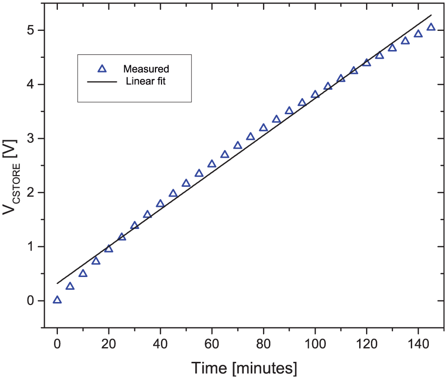
Figure 3 shows the voltage in $C_{\mathrm{store}}$ experimentally measured as a function of time for the circuit presented in Figure 2. The voltage was measured during the charging of a 1-F $C_{\mathrm{store}}$ supercapacitor when a voltage of 200 mV (best case in an environmental STEG) was applied to the $V_{\mathrm{TEG}}$ input of the DC–DC converter. From this plot, we can assume that the charge current is approximately constant and equal to 0.57 mA. This means that a totally discharged 1-F $C_{\mathrm{store}}$ supercapacitor requires approximately 145 min to be fully charged from 0 to 5 V.

Figure 3.

Measured value of the voltage in $C_{\mathrm{store}}$ as a function of time.

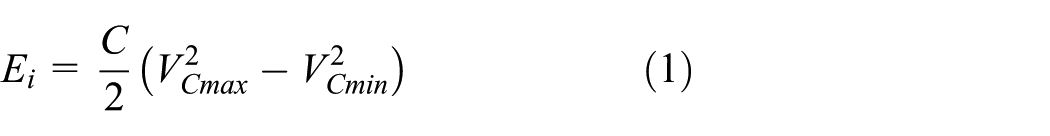
The usual technique to measure the energy stored in $C_{\mathrm{store}}$ is to charge and discharge it, several times, between two voltage levels and then calculate the electrical energy stored in each charge cycle. If we design a circuit that allows a capacitor initially charged with a voltage $V_{\mathrm{Cmin}}$ to charge up to a high level $V_{\mathrm{Cmax}}$ , we can write the energy $E_i$ stored during this charging cycle as follows

$$E_i=\frac{C}{2}(V_{\mathrm{Cmax}}^2-V_{\mathrm{Cmin}}^2)$$

(1)

If this charge/discharge measuring methodology is applied on a sunny day (where the 200 mV is available at the input of the DC–DC converter during 10 h), with $V_{\mathrm{Cmin}}=1.0$ V and $V_{\mathrm{Cmax}}=5.0$ V, by consulting the charging data from Figure 3, we conclude that the supercapacitor will complete one charging cycle in approximately 117 min. Thus, during 10 h, it will be necessary to discharge the supercapacitor five times.

However, supercapacitors cannot supply large currents and, for example, a 1-F state-of-the-art supercapacitor (EECS5R5H105; Panasonic) can be discharged with a maximum current of 1 mA. This imposes a problem to the proposed charge–discharge methodology. Discharging a 1-F supercapacitor from 5 V down to 1 V with a constant current $I_d=1$ mA will take approximately 67 min and, during this time, the harvested energy which would be stored in $C_{\mathrm{store}}$ will not be measured.

Developed circuit

To eliminate this error, the circuit presented in Figure 4, which has two supercapacitors ( $C_1$ and $C_2$ ), was developed. A complementary metal oxide semiconductor (CMOS) single-pole, double-throw switch $S{w}_1$ (ADG819; Analog Devices), controlled by the port P1.0 of the microcontroller MSP430F2122 (Texas Instruments), is used to select which supercapacitor is connected to $D_1$ .

Figure 4.

Developed measurement circuit.

During the charge period of $C_1$ , the switch $S{w}_1$ connects $D_1$ to $C_1$ , and during the time when $C_1$ is discharged, $S{w}_1$ connects $D_1$ to the auxiliary storage element, supercapacitor $C_2$ . Thus, during the period when $C_1$ is being discharged, the energy that cannot be stored in $C_1$ is stored in $C_2$ .

Since the maximum $\mathrm{dV}/\mathrm{dt}$ rate in the supercapacitors ( $C_1$ and $C_2$ ) is 1 mV/s (discharging the 1-F supercapacitor with a current of 1 mA), we make one A/D conversion at every 10 s, and the maximum error in the measurement of the supercapacitor voltage due to this slow sampling rate is only 10 mV.

It is important to note that the voltage in $V_{\mathrm{store}}$ can reach 5.25 V and the full-scale voltage of the internal A/D converter of the microcontroller is 1.2 V, so it is necessary to divide the voltages $V_{\mathrm{Cstore}}$ and $C_2$ before connecting them to the A/D input. This is done by $A_1$ , $A_2$ , and the resistor dividers $R_a-R_b$ and $R_c-R_d$ . $A_1$ and $A_2$ are 5 pA ultra-low input bias current op-amps (LT6004; Texas Instruments), so they will neither discharge the storage supercapacitors nor introduce measurement errors.

Measurement algorithm

The measurement algorithm is as follows. After the battery is connected to the system, the microcontroller begins a start-up sequence, preparing the circuit to begin the energy measurement routine. The $V_{\mathrm{TEG}}$ input of the DC–DC converter is connected to an external power supply with 500 mV in its output.

The microcontroller sets output P1.1 and P1.2 to “1,” so that transistors $Q_1-Q_2$ and $Q_3-Q_4$ are cut-off. Next, the microcontroller connects switch $S{w}_1$ to the position where $C_{\mathrm{store}}$ is allowed to be charged through $D_1$ , and the $A/D_1$ channel of the internal 10 bits A/D converter starts to read the voltage in $C_1$ .

$A/D_1$ monitors the voltage in $C_1$ until it reaches 2.0 V and then the microcontroller switches $S{w}_1$ to the position where $C_2$ is allowed to charge through $D_1$ . Now, the $A/D_2$ channel starts reading the voltage in $C2$ until it reaches 2.0 V. When this situation is reached, LED $L{D}_1$ is turned on by the microcontroller, indicating that the 500-mV power supply has to be disconnected from the $V_{\mathrm{TEG}}$ input of the DC–DC converter. A timing diagram showing the voltage sequencing and the charging of $C_1$ and $C_2$ is shown in Figure 5.

Figure 5.

Timing diagram of the first step of the start-up sequence.

After LED $L{D}_1$ is turned on, the microcontroller waits for 10 s (allowing for the disconnection of the power supply) and then starts the last step of the start-up sequence. The last step consists of forcing the initial conditions for both $C_1$ and $C_2$ . The microcontroller sets P1.1 to “0,” biasing, through $Q_3$ , the reference voltages $V_{\mathrm{ref}1}$ (LM385-1.2; Texas Instruments) and forcing the discharge of $C_1$ with the collector current of $Q_4$ , which is given by $I_{C4}=(V_{\mathrm{ref}1}-V_{\mathrm{BE}1})/R6$ .

Again $A/D_1$ monitors the voltage in $C_1$ until it reaches $V_{\mathrm{Cmin}}=1.0$ V when the current in $Q_4$ is immediately cut by setting P1.1 to “1.” The same procedure is applied with P1.2, $Q_1$ , $Q_2$ , and $A/D_2$ until $C_2$ voltage is equal to $V_{\mathrm{Cmin}}=1.0$ V. After the voltage in both capacitors is equal to $V_{\mathrm{Cmin}}=1.0$ V, $L{D}_1$ turns off, indicating that the start-up sequence is finished. A timing diagram showing the voltage sequencing and the discharging of $C_1$ and $C_2$ to $V_{\mathrm{Cmin}}=1.0$ V is shown in Figure 6.

Figure 6.

Timing diagram of the final step of the start-up sequence.

This finishes the start-up sequence and prepares the system to measure the energy available in the $V_{\mathrm{store}}$ terminal of the DC–DC converter when powered by a STEG energy harvesting system.

Energy measurement phase

After the start-up sequence is finished, the system starts measuring the total energy which can be stored by the STEG harvesting system. The switch $S{w}_1$ is positioned to connect $D_1$ to $C_1$ , and when the system is connected to a STEG, $C_1$ starts to charge from its initial condition $V_{\mathrm{Cmin}}=1.0$ V. Simultaneously, $A/D_1$ monitors the voltage in $C_1$ (once every 10 s) until it reaches $V_{\mathrm{Cmax}}=5.0$ V when $S{w}_1$ disconnects $D_1$ from $C_1$ and connects $D_1$ to $C_2$ .

Then, $C_2$ starts to charge, a counter $N_{C1}$ is increased (indicating that $C_1$ has completed one charging cycle), and the value of the counter $N_{C1}$ is written to the SD card. After $S{w}_1$ changes from $C_1$ to $C_2$ , P1.1 is set to “0,” and $Q_4$ starts to discharge $C_1$ . Now, we have $C_1$ being discharged (and monitored by $A/D_1$ ) and $C_2$ being charged (and monitored by $A/D_2$ ).

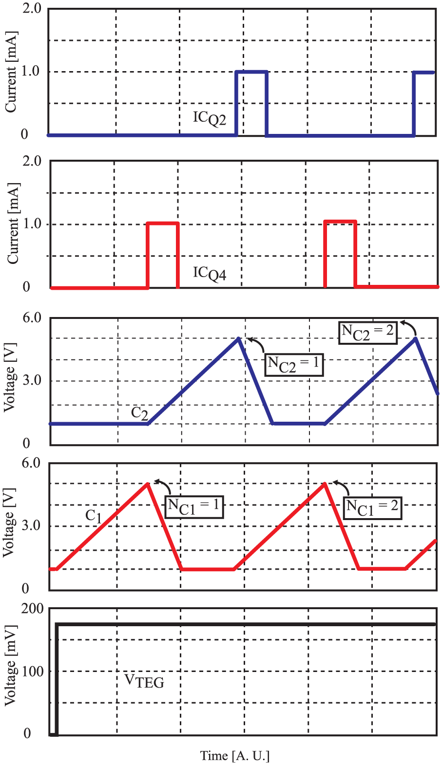
When $C_1$ reaches its initial condition $V_{\mathrm{Cmin}}=1.0$ V, P1.1 is set to “1,” turns off $Q_4$ , and is held in this position until a new cycle starts. The new cycle starts when $C_2$ reaches $V_{\mathrm{Cmax}}=5.0$ V, switch $S{w}_1$ changes back to $C_1$ , counter $N_{C2}$ is incremented and written to the SD card, and the discharging of $C_2$ is started by $Q_2$ . This alternate cycle repeats as long as the system is left running. A timing diagram showing the charge/discharge sequence of $C_1$ and $C_2$ between $V_{\mathrm{Cmax}}=5.0$ V and $V_{\mathrm{Cmin}}=1.0$ V is shown in Figure 7.

Figure 7.

Timing diagram of the charge/discharge sequence of $C_1$ and $C_2$ .

To remove the SD card safely, a manual switch Sm in the measurement circuit PCB (printed circuit board) is used to interrupt the program, write to the SD card the last value of the voltage $V_{\mathrm{last}}$ of the capacitor which is being charged ( $C_1$ or $C_2$ ), and stop any communication between the microcontroller and the SD card controller. After Sm is pressed and all the data are written to the SD card, and the communication between the microcontroller and the SD card is interrupted, the program is halted and LED $L{D}_2$ turns on indicating that the SD card can be safely removed.

Since the energy stored by $C_1$ and $C_2$ in each charging cycle is given by equation (2), with $C_1=C_2=C$ , it is possible to calculate the total energy stored by the energy harvesting system during the measurement period simply by

$$E_{\mathrm{total}}=E_{\mathrm{cycles}}+E_{\mathrm{last}}$$

(2)

where

$$E_{\mathrm{cycles}}=\frac{C}{2}(N_{C1}+N_{C2})(V_{\mathrm{Cmax}}^2-V_{\mathrm{Cmin}}^2)$$

(3)

and

$$E_{\mathrm{last}}=\frac{C_{(1,2)}}{2}({V_{\mathrm{last}}}^2-V_{\mathrm{Cmin}}^2)$$

(4)

Experimental results

Operation of the measurement circuit

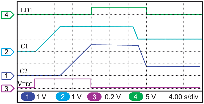
A prototype of the measurement system was implemented and tested in laboratory, with the values of $C_1$ and $C_2$ reduced to 1000 µF in order to accelerate the measurements. Figure 8 presents the measured voltages during the start-up sequence of the system.

Figure 8.

Measured voltages during start-up sequence.

After a pre-charge of the capacitors to 2.0 V, the LED $L{D}_1$ turns on, indicating that the power supply must be disconnected from the input of the DC–DC converter and the next phase of the start-up sequence can be initiated. Supercapacitors $C_1$ and $C_2$ are discharged (first $C_1$ and then $C_2$ ) to 1.0 V, 10 s after LED $L{D}_1$ turns on.

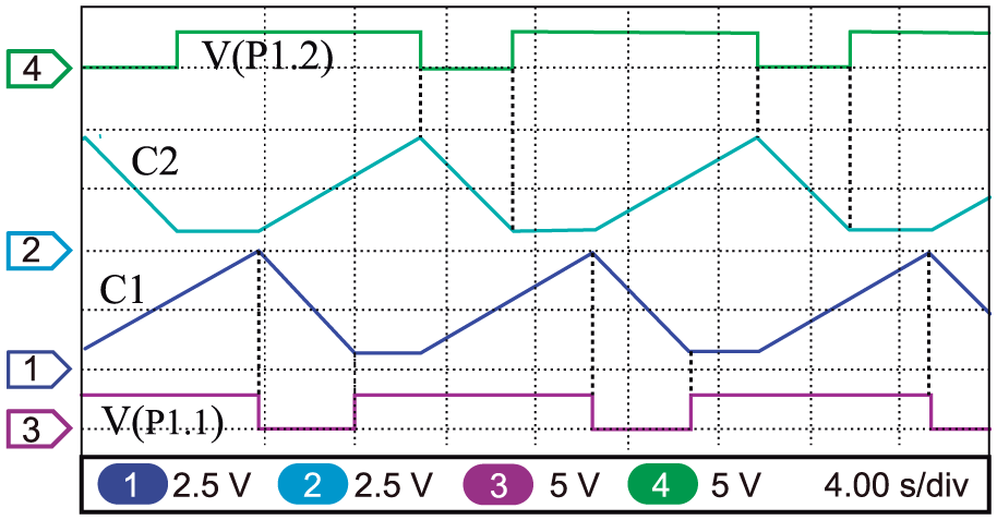
Figure 9 displays a plot of the measured voltages in $C_1$ and $C_2$ during the regular operation of the circuit with a constant 190 mV $V_{\mathrm{TEG}}$ input applied to the DC–DC converter. The voltages $V(P1.1)$ and $V(P1.2)$ were measured at the output pins of the microcontroller. As we can observe, the capacitors $C_1$ and $C_2$ are correctly charged and discharged alternately between $V_{\mathrm{Cmax}}$ and $V_{\mathrm{Cmin}}$ , as required for the proper operation of the system.

Figure 9.

Measured voltages during energy measurement phase.

Comparison of the single- and dual-capacitor measurement techniques

In order to compare the measured results from both techniques (the single capacitor used in Dias et al. ¹⁴ and the dual capacitor proposed in this article), various measurements were performed. In the tests, various constant input voltages $V_{\mathrm{TEG}}$ (from 35 to 180 mV) were applied to the DC–DC converter and, for each input voltage, the system was left running for 60 min. At the end of the 60-min period, the energy which could be stored in the supercapacitor was calculated. The first test was made with the dual capacitor circuit presented in Figure 4. For testing the single-capacitor technique, the same circuit was used, but the firmware of the system was modified in order to make the section comprising $C_2$ and its discharging circuit ( $Q_1,Q_2,V_{\mathrm{ref}1}$ ) inactive.

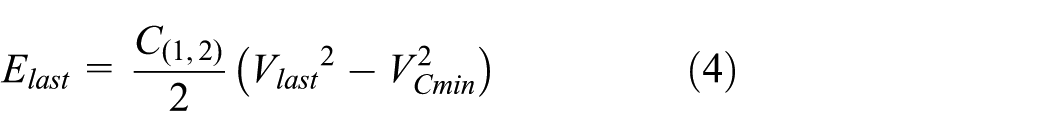
Another important modification was regarding the charge/discharge of $C_1$ . The firmware was changed in order to have $C_1$ continuously charged/discharged between $V_{\mathrm{Cmax}}=5$ V and $V_{\mathrm{Cmin}}=1$ V. The total number of charging cycles $N_{C1}$ and the last voltage in $C_1$ (at the exact moment the measurement period of 60 min is over) are stored in the microcontroller. The energy is calculated using equations (2)–(4), but with $N_{C2}=0$ .

The energy measured with both techniques is shown, as a function of the $V_{\mathrm{TEG}}$ input applied to the DC–DC converter, in the plot presented in Figure 10. The difference in the results of the energy measured with the two techniques is because, for the single-capacitor technique, during the time that $C_1$ is being discharged, the energy furnished by the DC–DC converter is not being measured.

Figure 10.

Energy furnished by the DC–DC converter for the single- and dual-capacitor techniques as a function of the $V_{\mathrm{TEG}}$ .

Neglecting the errors due to the A/D converter and the mismatches between the discharging currents $I_{C4}$ and $I_{C2}$ , we can assume that the energy measured with the dual-capacitor technique is correct and therefore calculate the percentage error $E(\%)$ between the two techniques. In Figure 11, the calculated percentage error $E(\%)$ between the two techniques is presented, and one can observe that for low-input voltages ( $V_{\mathrm{TEG}}<60$ mV), the single-capacitor technique leads to small measurement errors (lower than 6%), but when $V_{\mathrm{TEG}}$ increases, the measurement error with the single-capacitor technique increase up to 33% when $V_{\mathrm{TEG}}=180$ mV.

Figure 11.

Measured percentage error $E(\%)$ between single- and dual-capacitor measurement techniques as a function of the $V_{\mathrm{TEG}}$ .

Conclusion

A circuit to accurately measure the amount of thermal energy converted to electrical energy by a STEG and used to charge a supercapacitor storage element was designed, implemented, and tested. A microcontroller-based circuit is used to charge and discharge alternately two supercapacitors between two voltage levels $V_{\mathrm{Cmax}}$ and $V_{\mathrm{Cmin}}$ and to count the number of charge cycles of each of the supercapacitors. The total number of charging cycles of each supercapacitor is written to an SD card and, since the energy stored in each charging cycle is well known, the energy storage capacity in the STEG energy harvesting module under test is accurately measured. We observed that for low-input voltages ( $V_{\mathrm{TEG}}<60$ mV), the single-capacitor technique leads to small measurement errors (lower than 6%). However, when $V_{\mathrm{TEG}}$ increases to $V_{\mathrm{TEG}}=185$ mV, the dual capacitor measurement technique eliminates an error of 33% which is present in the single-capacitor measurement technique.