Analytical model for predictable contact in intermittently connected cognitive radio ad hoc networks

Abstract

In this article, an analytical model for predictable contact between two cognitive users in the intermittently connected cognitive radio ad hoc networks is proposed. The salient feature of the model is that it establishes a relationship between contact availability and the intermittently connected cognitive radio ad hoc network design parameters including cognitive user transmission range, velocity of cognitive user, direction of cognitive user, velocity of primary user, direction of primary user, and interference radius of primary user. However, a detailed analytical model is not available in the literature up to now. In particular, the relationship between contact availability and interference radius of primary user has not been derived in previous models. To research the contact availability, the concept of contact degree is first proposed to quantify the probability of contact availability between two cognitive users. In addition, the formulation for the contact degree between two cognitive users from different cases is illustrated in detail in this article. Under the contact degree scenario, the continuous effective contact time is derived to examine the communication duration of cognitive users based on the modified random walk mobility model. Finally, the simulation results demonstrate the effectiveness of the proposed analytical model for predictable contact in the intermittently connected cognitive radio ad hoc networks.

Introduction

Cognitive radio (CR) or dynamic spectrum access ¹ has newly emerged as a promising solution to improve the spectrum utilization by allowing unlicensed cognitive users (CUs) to access the idle licensed spectrum. In a CR network, CUs can periodically sense the licensed spectrum and opportunistically access the spectrum holes or spectrum opportunities (SOPs) unoccupied by primary users (PUs). In addition, CUs can further form an infrastructure-based CR network or a multi-hop ad hoc network without the support of fixed infrastructure. In a cognitive radio ad hoc network (CRANET), ² CUs can only access the SOPs in a distributed fashion by seeking to underlay, overlay, or interweave their signals with those of existing PUs without significantly impacting their communications. However, the potential of high mobility and low node density of CUs as well as the limitation of spectrum availability in CRANETs may result in the intermittent connectivity in such networks.^3,4 In this scenario, the CUs cannot turn to be in the condition of continuous connections. Moreover, the network topology may be subject to frequent interruptions due to the intermittent connectivity of the CU links. In particular, there is no guaranteed continuous end-to-end multi-hop path in the intermittently connected CRANETs.

In recent years, the architecture of a class of challenged networks, known as delay- and disruption-tolerant networking (DTN) architecture,^5,6 has been regarded as a promising approach to provide an overlay network for the highly challenged networks characterized with intermittent connectivity, frequent partitions, high latency, and so on. Therefore, it is uncovered that the intermittently connected CRANETs can be viewed as a typical scenario of DTNs.^3,4 From a routing perspective, the intermittently or partially connected dynamic topologies of the intermittently connected CRANETs will lead to the break of the established end-to-end paths. Along a path from source to destination, every link break may cause the path break. Then, this path needs to be either locally repaired by finding another link if possible or globally replaced by a new path through rerouting. Route repair or rerouting will induce much energy consumption, waste the scarce radio resources, and degrade end-to-end network performance including system throughput and transmission delay. ⁷ Remark that an available link connects two CUs in the intermittently connected CRANETs if and only if there exists a contact between them. In particular, a contact can be viewed as a communication opportunity during which two adjacent CUs can communicate with each other. Previous works mainly focus on three types of contacts including scheduled, predictable and opportunistic contacts in DTNs. ⁸ In a sense, a contact may be very precise or even can be predicted accurately. ⁹ In other words, the predictable contact between two adjacent CUs relies on the predictions of the likely contact times and durations based on the history of previously observed contacts.

A large number of analytical models or algorithms for the predictable contact, such as Zhuo et al., ¹⁰ Yuan et al., ¹¹ Sun et al., ¹² Yu et al., ¹³ and Guo and Chan, ¹⁴ are available for the contact availability prediction in DTNs. In Zhuo et al., ¹⁰ a practical contact duration aware replication algorithm (DARA) is proposed, which operates in a fully distributed manner and also reduces the computational complexity of the corresponding algorithm. Specifically, the different types of contacts in bus-based DTNs are characterized, and the effects of the radio range on contact duration are further examined, aiming to gain new insights for routing algorithms in practical scenario. In Yuan et al., ¹¹ a model based on a time-homogeneous semi-Markov process (TH-SMP) model is used to predict the probability distribution of the contact time as well as the probability of contact in the future. In Sun et al., ¹² by processing the history contact data with autoregression moving average (ARMA) model of time series analysis theory, the start time and the duration of future contact between specified nodes can be predicted without needing to know the movement model of the nodes. In Yu et al., ¹³ based on the fine-grained contact statistics, a greedy forwarding scheme is designed by combining the advantages of contact duration–based forwarding and quota-based routing. In Guo and Chan, ¹⁴ an algorithm entitled Plankton uses a combination of both short-term bursty contacts and long-term association-based statistics for contact prediction. In addition, Plankton dynamically adjusts replication quotas based on estimated contact probabilities. The referred analytical models above for predictable contact mainly focus on the prediction of contact duration, contact times, or contact probability, which are used to measure the contact availability in DTNs. Because the intermittently connected CRANETs have some characteristics which are different from DTNs. Foremost, the CUs make full use of the existing SOPs without causing harmful interference or collisions to the PUs in the intermittently connected CRANETs. However, the nodes have the equal right to utilize the available spectrum in DTNs. Furthermore, the relationship between contact availability and interference radius of PU has not been derived in previous analytical models. Therefore, the referred analytical models^10–14 as stated above for the predictable contact in DTNs are not completely suitable for the intermittently connected CRANETs.

In this article, an analytical model for predictable contact in the intermittently connected CRANETs is proposed. To facilitate the research of contact availability, a classification for predictable contact paradigm between two CUs including contact, non-contact, and effective contact is given. Then, the probability of continuous effective contact between two CUs is defined as contact degree. Subsequently, the contact degree between two CUs is characterized from different cases in detail. Furthermore, many insights into the impact of the contact degree between two CUs on the end-to-end network performance such as throughput and delay are presented. Next, under the constraint of contact degree, the concept of continuous effective contact time used to measure the communication duration between two CUs is proposed. By means of infinitesimal calculus, the continuous effective contact time is formulated using the modified random walk mobility model as a reference. In addition, the mean value of the continuous effective contact time can be obtained as well. Furthermore, the mean duration for CUs beyond the interference range of a PU is also derived. Simulation results indicate that the presented analytical model for predictable contact achieves close-to-optimal performance.

The remainder of this article is organized as follows. Section “System model” overviews the network model and mobility model. Section “Analytical model” proposes the analytical model which mainly involved the concept of contact degree. Section “Continuous effective contact time analysis” presents an important metric called continuous effective contact time. The simulation results are shown in section “Simulation results.” Finally, section “Conclusion” concludes the article by summarizing our results.

System model

Network model

Assume there is an intermittently connected underlay CRANETs serving N CUs with bidirectional symmetrical links. In this scenario, there are two PUs that send data to the primary base station in a set of licensed channels through the cellular primary network. The independent and identically distributed alternating ON-OFF process is employed to model the occupation time length of PU in licensed channels. Due to the random nature of PUs’ traffic and PUs’ dynamic, the available channels to each CU may only be a subset of licensed channels. Note that CUs can access the subset of licensed channels only when the interference temperature of PU is lower than the threshold that PU can tolerate. Through the local spectrum sensing, each CU dynamically accesses a channel to deliver data but can only work on one of the available channels temporarily. Thus, CUs are self-organized into an intermittently connected CRANETs. Let $S=\{1,2,\dots ,N\}$ denote the set of CUs with the same transmission radius r. In addition, it is assumed that the interference radius of PU is R. Remark that CU m and CU n, for $n,m\in S$ , can successfully transmit their traffic if and only if the following constraints that need to be taken into account:

• C1: there exists at least one common available channel between CU m and CU n;

• C2: the Euclidean distance between CU m and CU n should be lower than r;

• C3: CU m and CU n are both out of the interference radius R of PU.

Mobility model

The proposed analytical model for predictable contact in the intermittently connected CRANETs is based on the modified random walk mobility model. ¹⁵ It is assumed that CU n can move freely in the two-dimensional borderless plane. After CU n moves from its current position to a new position by randomly choosing a velocity and a direction during a period of time, it selects another velocity and direction to travel. The period of time above is defined as an epoch. The ith epoch length is independent and identically distributed (iid) and exponentially distributed. During ith epoch, CU n moves in a straight line with the velocity $V_n^i$ and the direction ${\theta }_n^i$ , for, $V_n^i\in [a,b]$ and ${\theta }_n^i\in [0,2\pi ]$ , where a and b are the positive constants. The velocity and direction obey arbitrary random distribution. In addition, the velocity, direction, and epoch length are uncorrelated with each other. Note that it will not change the velocity and direction until the next epoch. Not only the mobility among CUs is uncorrelated but also the contact break is independent.

Analytical model

In this section, several kinds of predictable contact are introduced. To facilitate the research of predictable contact, the concept of contact degree is also presented. Next, the formulation for the contact degree and a detail analysis from different cases are both given. Considering the mobility of CUs and the possible difference of epoch in the intermittently connected CRANETs, CU n may remain the velocity and direction constant during a certain epoch, while CU m may change its velocity and direction. For the purposes of discussion, the common epoch paradigm is illustrated as follows.

Definition 1 (common epoch)

The common epoch is the duration in which both CU m and CU n remain their velocities and directions constant.

According to the characteristics of exponential distribution, the common epoch is exponential distribution with parameter $({\lambda }^{*}{)}^{-1}$ which is similarly used in McDonald and Znati ¹⁶ and Jiang. ¹⁷ Thus, its probability distribution function can be expressed as

$$E(x)=P\{\mathrm{common\; epoch}⩽x\}=1-e^{-{\lambda }^{*}x}$$

(1)

where ${\lambda }^{*}={\lambda }_m+{\lambda }_n$ . For simplicity, it is assumed that ${\lambda }_m={\lambda }_n=\lambda$ . Specifically, ${\lambda }^{*}=2\lambda$ . Hence, $E(x)$ can be rewritten as the following form

$$E(x)=1-e^{-2\lambda x}$$

(2)

Moreover, the probability density function can be further written as

$$f(x)=2\lambda e^{-2\lambda x}$$

(3)

As CU m and CU n have different missions and service requirements, the duration in which the CU m and CU n remain their velocities and directions constant may be different. Let $T_m$ and $T_n$ denote the duration of CU m and CU n, respectively. For analytical simplicity, let $T=min\{T_m,T_n\}$ . Then, let time instant $t_0$ denote the initial time, after which both CU m and CU n remain their velocities and directions constant. Without loss of generality, let $t_0=0$ .

Definition 2 (contact, non-contact, effective contact)

The contact between CU m and CU n is defined as a communication opportunity if and only if C1 and C2 are both satisfied. The non-contact between CU m and CU n is defined as the case that there is no communication opportunity. The effective contact between CU m and CU n is defined as an effective communication opportunity if and only if C1, C2, and C3 are all satisfied simultaneously.

Definition 3 (contact degree)

Assume that CU m and CU n are in effective contact at initial time instant $t_0$ , the contact degree between CU m and CU n at time instant t is represented by the probability that CU m and CU n keep continuous effective contact from time instant $t_0$ to time instant t.

Let $C{D}_{m,n}(t)$ denote the probability that CU m and CU n be in continuous effective contact at time instant t. Note that $C{D}_{m,n}(t)\in [0,1]$ . If $C{D}_{m,n}(t)=0$ , it means that CU m and CU n are in non-contact from $t_0$ to t. If $C{D}_{m,n}(t)=1$ , it means that CU m and CU n are in continuous effective contact from $t_0$ to t. Otherwise, $0<C{D}_{m,n}(t)<1$ , it means that CU m and CU n are not always in effective contact from $t_0$ to t.

According to Definition 3, the contact degree between CU m and CU n at time instant t is formally given as

$$\begin{array}{c}C{D}_{m,n}(t)=\{\mathrm{CU}m\mathrm{and\; CU}n\mathrm{keep\; continuous\; effective\; contact\; from\; time\; instant}{t}_0\mathrm{to}t|\hfill \\ \mathrm{CU}m\mathrm{and}\mathrm{CU}n\mathrm{are\; in\; effective\; contact\; at\; time\; instant}{t}_0\}\hfill \end{array}$$

(4)

It is assumed that the predictable continuous effective contact time between CU m and CU n is denoted by $\mathrm{CC}{T}_{m,n}$ at time instant $t_0$ . Let T denote the duration that both CU m and CU n remain their velocities and directions constant at first time. Then, based on the current positions, velocities and directions of CU m and CU n at time instant $t_0+T$ , a new continuous effective contact time represented by ${\mathrm{CCT}}_{m,n}^2$ can be predicted. For convenience, let $\delta (m,n)$ replaces ${\mathrm{CCT}}_{m,n}^2$ . Next, let $\eta$ denote the duration that CU m and CU n both remain their velocities and directions constant after time instant $t_0+T$ . According to the above assumptions and the constraints of t, $\mathrm{CC}{T}_{m,n}$ , and T, $C{D}_{m,n}(t)$ can be calculated from different cases. In Figure 1, the value of time instant t varies with the vertical dotted line, which can slide on the abscissa axis. Then, an analysis is given as the following cases.

Figure 1.

The prediction analysis of contact degree under different cases: (a) $t⩽\mathrm{CC}{T}_{m,n}⩽T$ , (b) $T>t>\mathrm{CC}{T}_{m,n}$ , (c) $t⩽T⩽\mathrm{CC}{T}_{m,n}$ , (d) $t⩽T⩽\delta (m,n)$ , and (e) $t>\delta (m,n)>T$ .

Case 1: $T⩾\mathrm{CC}{T}_{m,n}$

Case 1 illustrates that both CU m and CU n remain their velocities and directions constant after the predictable continuous effective contact time of $\mathrm{CC}{T}_{m,n}$ . Then, this case can be divided into two sub-cases according to the constraints of t and $\mathrm{CC}{T}_{m,n}$ .

Theorem 1

Consider the predictable continuous effective contact time $\mathrm{CC}{T}_{m,n}$ given that $t⩽\mathrm{CC}{T}_{m,n}⩽T$ , then the contact degree $C{D}_{m,n}(t)=1$ .

Proof

If $t⩽\mathrm{CC}{T}_{m,n}⩽T$ , as shown in Figure 1(a), CU m and CU n remain their velocities and directions constant before the predictable time instant $t_0+T$ . Thus, the predictable continuous effective contact time $\mathrm{CC}{T}_{m,n}⩾t$ . Hence, CU m and CU n are in effective contact.

Theorem 2

Consider the predictable continuous effective contact time $\mathrm{CC}{T}_{m,n}$ given that $t>\mathrm{CC}{T}_{m,n}$ , then the contact degree $C{D}_{m,n}(t)=0$ .

Proof

If $t>\mathrm{CC}{T}_{m,n}$ , as shown in Figure 1(b), CU m and CU n are in non-contact at time instant $t_0+\mathrm{CC}{T}_{m,n}$ which is ahead of the predictable time instant $t_0+t$ .

Case 2: $T⩽\mathrm{CC}{T}_{m,n}$

Case 2 illustrates that CU m and CU n have changed their velocities and directions before the first possible non-contact of the two CUs. Hence, CU m and CU n may be in contact.

Theorem 3

Consider the duration T given that $t⩽T$ , then the contact degree $C{D}_{m,n}(t)=1$ .

Proof

If $t⩽T$ , as shown in Figure 1(c), the proof is similar to the case of $t⩽\mathrm{CC}{T}_{m,n}⩽T$ . Apparently, CU m and CU n are in effective contact.

If $t>T$ , as shown in Figure 1, CU m and CU n keep effective contact before time instant $t_0+t$ . Therefore, it is necessary to discuss whether CU m and CU n keep effective contact or not in the internal $[t_0+T,t_0+t]$ whose length is within the period of time $t-T$ . Now, the case that CU m and CU n changing their velocities and directions two or more times should be considered. Therefore, it can be concretely divided into the following two sub-cases.

Theorem 4

If $\eta ⩾t-T$ , let ${\mathrm{CD}}_{m,n}^1(t)$ denote the contact degree between CU m and CU n. If $\eta <t-T$ , let ${\mathrm{CD}}_{m,n}^2(t)$ denote the contact degree between CU m and CU n. Consider the duration T given that $t⩽T⩽\delta (m,n)$ , then the contact degree $C{D}_{m,n}(t)$ can be expressed as

$$\begin{array}{l}C{D}_{m,n}(t)=P\{\eta ⩾t-T\}\times C{D}_{m,n}^1(t)\\ +P\{\eta <t-T\}\times C{D}_{m,n}^2(t)\end{array}$$

(5)

Proof

According to whether the value of the random variable $\eta$ is greater than $t-T$ or not, the contact degree can be obtained, which is equal to the sum of conditional probability of the two cases. If the period of time $\eta$ during which CU m and CU n remain their velocities and directions constant can reach to $t-T$ , then CU m and CU n will keep effective contact in duration $t-T$ , that is, ${\mathrm{CD}}_{m,n}^1(t)=1(\eta ⩾t-T)$ . Otherwise, the other case that CU m and CU n changing their velocities and directions three or more times should be considered. In this case, let $C_{\mathrm{av}}$ denote the contact degree, that is, ${\mathrm{CD}}_{m,n}^2(t)=C_{\mathrm{av}}(\eta <t-T)$ . According to the definition of conditional probability, the contact degree $C{D}_{m,n}(t)$ in equation (5) can be further rewritten. The diagram is shown in Figure 1(d).

According to equation (2), equation (5) can be further written as

$$C{D}_{m,n}(t)=e^{-2\lambda (t-T)}+(1-e^{-2\lambda (t-T)})\times C_{\mathrm{av}}$$

(6)

Theorem 5

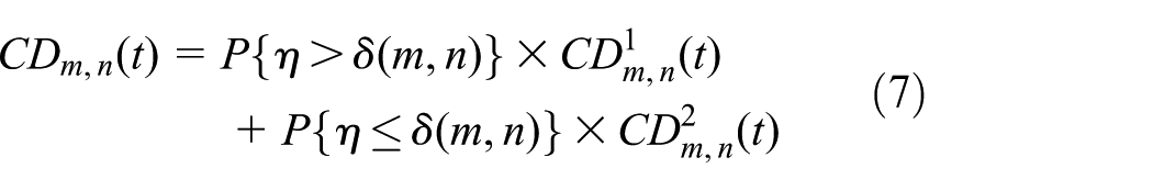
If $\eta ⩾\delta (m,n)$ , let ${\mathrm{CD}}_{m,n}^1(t)$ denote the contact degree between CU m and CU n. If $\eta <\delta (m,n)$ , let ${\mathrm{CD}}_{m,n}^2(t)$ denote the contact degree between CU m and CU n. Consider the duration T given that $t-T>\delta (m,n)$ , then the contact degree $C{D}_{m,n}(t)$ can be expressed as

$$\begin{array}{l}C{D}_{m,n}(t)=P\{\eta >\delta (m,n)\}\times C{D}_{m,n}^1(t)\\ +P\{\eta ⩽\delta (m,n)\}\times C{D}_{m,n}^2(t)\end{array}$$

(7)

Proof

The proof is similar to the proof of Theorem 4. According to whether the value of the random variable $\eta$ is greater than $\delta (m,n)$ or not, the contact degree between CU m and CU n can be obtained, which is equal to the sum of conditional probability of the two cases. If CU m and CU n both remain their velocities and directions constant in the duration $\delta (m,n)$ , they will be in non-contact, that is, ${\mathrm{CD}}_{m,n}^1(t)=0(\eta ⩾\delta (m,n))$ . Otherwise, it is similar to the Theorem 4, that is, ${\mathrm{CD}}_{m,n}^2(t)=C_{\mathrm{av}}(\eta <\delta (m,n))$ . According to the definition of conditional probability, the contact degree $C{D}_{m,n}(t)$ in equation (7) can be further rewritten. The diagram is shown in Figure 1(e).

According to equation (2), equation (7) can be rewritten as

$$C{D}_{m,n}(t)=(1-e^{-2\lambda \delta (m,n)})\times C_{\mathrm{av}}$$

(8)

Then, the possible cases after CU m and CU n change their velocities and directions two times should be considered. Let $C_{\mathrm{av}}$ denote the contact degree of the possible cases. Then, let $\eta$ denote the length of the second common epoch of CU m and CU n. If CU m and CU n change their velocities and directions two or more times, let $T_s$ denote the continuous effective contact time between CU m and CU n since time instant $t_0$ . Thus, let $C(\eta )$ denote the contact degree between CU m and CU n.

According to the idea proposed by Jiang, ¹⁷ $C(\eta )$ can be obtained as follows

$$C(\eta )=\frac{T_s}{t}=\frac{T+\eta +(t-T-\eta )e^{-2\lambda (t-T-\eta )}}{t}$$

(9)

As $\eta$ is a random variable, using the mean value $C(\eta )$ , $C_{\mathrm{av}}$ can be estimated as follows

$$C_{\mathrm{av}}=\underset{0}{\overset{t-T}{\int }}C(\eta )f(\eta )d\eta$$

(10)

According to equation (3), substituting equation (9) into equation (10), a new formula can be obtained as follows

$$C_{\mathrm{av}}=\frac{1+2\lambda t+e^{-2\lambda (t-T)}(-1-2\lambda t+2{\lambda }^2{(t-T)}^2)}{2\lambda t}$$

(11)

In equation (8), $\delta (m,n)$ represents the continuous effective contact time after CU m and CU n change their velocities and directions two times. However, the necessary information of the CUs, such as, the position, velocity and direction, are unknown. Consequently, the precise value of $\delta (m,n)$ cannot be obtained. In fact, we can replace $\delta (m,n)$ with the mean value $\overline{\delta }(m,n)$ .

Continuous effective contact time analysis

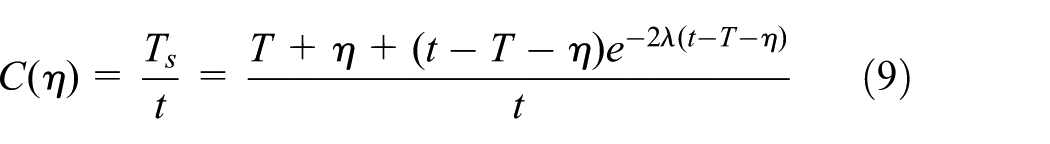
In this section, a formulation for the continuous effective contact time between CU m and CU n and a detailed analysis about the mean value of the continuous effective contact time are both given. It is assumed that the transmission radius of CU m and CU n are both r. Let $v_m$ and $v_n$ , respectively, denote the velocity of CU m and the velocity of CU n. In addition, the included angle between $v_m$ and $v_n$ is $\theta$ . Regard the movement of CU m and CU n as the movement of CU m relative to CU n. According to cosine law, their relative velocities can be obtained, that is, $V=\sqrt{v_m^2+v_n^2-2v_m{v}_n\cos \theta }$ . As the distance between CU m and CU n varies by $v_m$ , $v_n$ , $\theta$ and their common epoch. Let $D_{\mathrm{mn}}$ denote the current distance between CU m and CU n. Note that the current distance $D_{\mathrm{mn}}$ means the distance between CU m and CU n at some point. To describe the distribution characteristic of $D_{\mathrm{mn}}$ , the probability distribution function of $D_{\mathrm{mn}}$ is expressed as

$$F(D_{\mathrm{mn}})=(1-e^{-2\lambda x})\underset{-\infty }{\overset{+\infty }{\int }}\underset{-\infty }{\overset{+\infty }{\int }}\underset{0}{\overset{2\pi }{\int }}f(v_m,v_n,\theta )d{v}_{m}d{v}_{n}d\theta$$

(12)

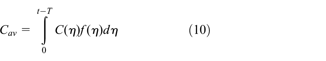
where $f(v_m,v_n,\theta )$ is the joint probability density function of the random variables $v_m$ , $v_n$ and $\theta$ . Since $v_m$ , $v_n$ and $\theta$ are mutually independent, their relationship can be expressed by $f(v_m,v_n,\theta )=f(v_m)\times f(v_n)\times f(\theta )$ . It should be noted that $f(v_m)$ , $f(v_n)$ , and $f(\theta )$ are, respectively, the probability density function of $v_m$ , $v_n$ , and $\theta$ . In particular, it is more important to obtain the aggregate distance of CU m moves with constant velocity and direction from the initial position to the boundary of the transmission range of CU n than the current distance between CU m and CU n. Let d denote the aggregate distance of CU m move out of the transmission range of CU n. Therefore, the continuous effective contact time between CU m and CU n $\mathrm{CC}{T}_{m,n}=d/V$ . Obviously, the initial position of CU n is uniformly distributed within the transmission range of CU m. In addition, the transmission range of CU m is a circle with radius r. The included angle $\theta$ of relative velocity obeys uniform distribution over $[0,2\pi ]$ . Hence, the random variable d obeys uniform distribution over $[0,2r]$ . Moreover, the mean value $\overline{\delta }(m,n)$ of $\mathrm{CC}{T}_{m,n}$ is equal to the mathematical expectation $E(\mathrm{CC}{T}_{m,n})$ . To be specific, $\overline{\delta }(m,n)=E(\mathrm{CC}{T}_{m,n})=E(d/V)$ . The random variables $v_m$ , $v_n$ , $\theta$ , and d are mutually independent. Furthermore, d and V are also independent with each other. Thus, $E(\mathrm{CC}{T}_{m,n})=E(d)\times E(1/V)$ . Considering that d obeys uniform distribution over $[0,2r]$ , $E(d)=(0+2r)/2=r$ . Hence, $E(1/V)$ can be formulated as

$$E\left(\frac{1}{V}\right)=\underset{0}{\overset{2\pi }{\int }}\underset{-\infty }{\overset{+\infty }{\int }}\underset{-\infty }{\overset{+\infty }{\int }}g(v_m,v_n,\theta )f(v_m,v_n,\theta )d{v}_{m}d{v}_{n}d\theta$$

(13)

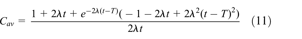
Therefore, the mean value $\overline{\delta }(m,n)$ of $\mathrm{CC}{T}_{m,n}$ can be expressed as

$$\begin{array}{l}\overline{\delta }(m,n)=(r-D_{mn0})\\ {\displaystyle \underset{0}{\overset{2\pi }{\int }}{\displaystyle \underset{-\infty }{\overset{+\infty }{\int }}{\displaystyle \underset{-\infty }{\overset{+\infty }{\int }}g(v_m,v_n,\theta )}}}f(v_m,v_n,\theta )d{v}_{m}d{v}_{n}d\theta \end{array}$$

(14)

where $D_{\mathrm{mn}0}$ is the initial distance of CU m to CU n, $g(v_m,v_n,\theta )=1/V$ . Taking into account the mobility model referred above, it is assumed that the velocity v obeys uniform distribution over $[a,b]$ and the included angle $\theta$ of relative velocity obeys uniform distribution over $[0,2\pi ]$ . Thus, $f(v)=1/(b-a)$ , $f(\theta )=1/2\pi$ . Furthermore, the mean value $\overline{\delta }(m,n)$ of $\mathrm{CC}{T}_{m,n}$ can be obtained as follows

$$\begin{array}{c}\overline{\delta }(m,n)=(r-D_{\mathrm{mn}0})\underset{0}{\overset{2\pi }{\int }}\underset{a}{\overset{b}{\int }}\underset{a}{\overset{b}{\int }}\frac{1}{\sqrt{v_m^2+v_n^2-2v_m{v}_n\cos \theta }}\times \frac{1}{b-a}\times \frac{1}{b-a}\times \frac{1}{2\pi }d{v}_{m}d{v}_{n}d\theta \hfill \\ =\frac{r-D_{\mathrm{mn}0}}{2\pi {(b-a)}^2}\underset{0}{\overset{2\pi }{\int }}\underset{a}{\overset{b}{\int }}\underset{a}{\overset{b}{\int }}\frac{1}{\sqrt{v_m^2+v_n^2-2v_m{v}_n\cos \theta }}d{v}_{m}d{v}_{n}d\theta \hfill \end{array}$$

(15)

To facilitate the research of the spatial relationships between the CUs and a PU, let $D_{\mathrm{mpu}}$ and $D_{\mathrm{npu}}$ , respectively, denote the current distance from CU m and CU n to a PU at some point. Remark that $F(D_{\mathrm{mpu}})$ and $F(D_{\mathrm{npu}})$ can be obtained by equation (12). The probability distribution function of $D_{\mathrm{mpu}}$ and $D_{\mathrm{npu}}$ are, respectively, expressed as

$$F(D_{\mathrm{mpu}})=(1-e^{-2\lambda x})\underset{-\infty }{\overset{+\infty }{\int }}\underset{-\infty }{\overset{+\infty }{\int }}\underset{0}{\overset{2\pi }{\int }}f(v_m,v_{\mathrm{pu}},\theta )d{v}_{m}d{v}_{\mathrm{pu}}d\theta$$

(16)

$$F(D_{\mathrm{npu}})=(1-e^{-2\lambda x})\underset{-\infty }{\overset{+\infty }{\int }}\underset{-\infty }{\overset{+\infty }{\int }}\underset{0}{\overset{2\pi }{\int }}f(v_n,v_{\mathrm{pu}},\theta )d{v}_{n}d{v}_{\mathrm{pu}}d\theta$$

(17)

where $f(v_m,v_{\mathrm{pu}},\theta )$ is the joint probability density function of the random variables $v_m$ , $v_{\mathrm{pu}}$ , and $\theta$ . Similarly, $f(v_n,v_{\mathrm{pu}},\theta )$ is the joint probability density function of the random variables $v_n$ , $v_{\mathrm{pu}}$ , and $\theta$ . Since $v_m$ , $v_n$ , $v_{\mathrm{pu}}$ , and $\theta$ are mutually independent, their relationship can be expressed by $f(v_m,v_{\mathrm{pu}},\theta )=f(v_m)\times f(v_{\mathrm{pu}})\times f(\theta )$ and $f(v_n,v_{\mathrm{pu}},\theta )=f(v_n)\times f(v_{\mathrm{pu}})\times f(\theta )$ . It should be noted that $f(v_m)$ , $f(v_n)$ , $f(v_{\mathrm{pu}})$ , and $f(\theta )$ are, respectively, the probability density function of $v_m$ , $v_n$ , $v_{\mathrm{pu}}$ , and $\theta$ . The CUs within the interference range of a PU at time instant $t_0$ will not be considered because the CUs impact the normal communication of a PU. Thus, the CUs beyond the interference range of a PU at time instant $t_0$ is just the focus of attention. Then, the duration of CUs beyond the interference range of a PU after time instant $t_0$ will be predicted. As illustrated in Figure 2(a), a CU moves to the other one and a CU moves to a PU in Figure 2(b).

Figure 2.

A sketch of the movement among CUs: (a) the mobility between CU nodes and (b) the mobility between CU node and PU node.

Let $\overline{\epsilon }(m,\mathrm{pu})$ denote the mean duration of CU m beyond the interference range of a PU. Then, $\overline{\epsilon }(m,\mathrm{pu})$ can be calculated as

$$\begin{array}{l}\overline{\epsilon }(m,pu)=\frac{D_{m0}-R}{2\pi {(b-a)}^2}\\ {\displaystyle \underset{0}{\overset{2\pi }{\int }}{\displaystyle \underset{a}{\overset{b}{\int }}{\displaystyle \underset{a}{\overset{b}{\int }}\frac{1}{\sqrt{v_m^2+v_{pu}^2-2v_m{v}_{pu}\cos \theta }}d{v}_{m}d{v}_{pu}d\theta }}}\end{array}$$

(18)

where $D_{m0}$ is the initial distance of CU m to a PU.

Similarly, let $\overline{\epsilon }(n,\mathrm{pu})$ describe the mean duration of CU n beyond the interference range of a PU. Hence, $\overline{\epsilon }(n,\mathrm{pu})$ can be formally written as follows

$$\begin{array}{l}\overline{\epsilon }(n,pu)=\frac{D_{n0}-R}{2\pi {(b-a)}^2}\\ {\displaystyle \underset{0}{\overset{2\pi }{\int }}{\displaystyle \underset{a}{\overset{b}{\int }}{\displaystyle \underset{a}{\overset{b}{\int }}\frac{1}{\sqrt{v_n^2+v_{pu}^2-2v_n{v}_{pu}\cos \theta }}d{v}_{n}d{v}_{pu}d\theta }}}\end{array}$$

(19)

where $D_{n0}$ is the initial distance of CU n to a PU.

Theorem 6

Let $T_e$ represent the minimum value of $\mathrm{CC}{T}_{m,n}$ . $T_e$ can be further expressed as

$$T_e=min\{\overline{\delta }(m,n),\overline{\epsilon }(m,\mathrm{pu}),\overline{\epsilon }(n,\mathrm{pu})\}$$

(20)

Proof

Considering the CUs’ interference to a PU and the movement between the CUs, the normal communication time among the CUs is the minimum value of the continuous contact time of the CUs and the time of the CUs do not interfere with a PU. That is, CUs should satisfy the definition of effective contact. Therefore, $T_e$ is the minimum value of $\overline{\delta }(m,n)$ , $\overline{\epsilon }(m,\mathrm{pu})$ , and $\overline{\epsilon }(n,\mathrm{pu})$ .

Simulation results

In this section, the performance of the analytical model is evaluated by contact degree and continuous effective contact time. It is convincing to verify the results’ validity of the contact degree by comparing it with the results of simulation experiments. The simulation environment is a two-dimensional unbounded space. In the simulation experiments, the CU’s transmission radius r, the average length of epoch, the PU’s interference radius R, and the velocities and directions of CUs are selected as a set of parameters. Next, 10 CUs and 2 PUs are randomly generated. Then, the time T during which the two CUs being in effective contact first remain their velocities and directions constant will be given. Let the CUs move as the modified random walk mobility model and gather the statistics of the real time of CUs being in continuous effective contact in the total simulation time. Finally, through a large number of independent repeated experiments and by utilizing the statistical method, the probability of CUs being in continuous effective contact until $\mathrm{CC}{T}_{m,n}$ in the realistic simulation environment can be obtained. Let $C{D}_{\mathrm{sim}}$ denote the probability of CUs being in continuous effective contact until $\mathrm{CC}{T}_{m,n}$ in the realistic simulation environment. In addition, the velocity obeys the uniform distribution over $[a,b]$ and the predictable moment is $\mathrm{CC}{T}_{m,n}$ . The abscissa represents the average length of common epoch, that is, ${\lambda }^{-1}$ , and the corresponding unit is second. The ordinate represents the contact degree. The parameter values of four simulation experiment scenarios are shown in Table 1.

Table 1.

The parameter values of four simulation experiment scenarios.

Scenario (a)	Scenario (b)	Scenario (c)	Scenario (d)
$r=100\mathrm{m}$	$r=100\mathrm{m}$	$r=250\mathrm{m}$	$r=250\mathrm{m}$
$R=65\mathrm{m}$	$R=65\mathrm{m}$	$R=65\mathrm{m}$	$R=65\mathrm{m}$
$a=0\mathrm{m}/\mathrm{s}$	$a=5\mathrm{m}/\mathrm{s}$	$a=0\mathrm{m}/\mathrm{s}$	$a=5\mathrm{m}/\mathrm{s}$
$b=10\mathrm{m}/\mathrm{s}$	$b=10\mathrm{m}/\mathrm{s}$	$b=10\mathrm{m}/\mathrm{s}$	$b=10\mathrm{m}/\mathrm{s}$

In Figure 3, it is effective to compare the results obtained by analytical model with the results of the simulation experiments, in order to examine the predicted performance of the contact degree $C{D}_{m,n}(t)$ at time instant $\mathrm{CC}{T}_{m,n}$ . Figure 3 shows the detailed properties about the contact degree and the average common epoch under different scenarios. In Figure 3, according to a large number of independent repeated experiments and the statistical method, the continuous effective contact time until $\mathrm{CC}{T}_{m,n}$ in the realistic simulation environment can be obtained, that is, 18.13546 s. In addition, it is observed clearly that the contact degree of many points trends very close to one. The results are consistent with equation (6) or equation (8), which is the sum of conditional probability. During the time 18.13546 s, the two CUs are in continuous effective contact. For instance, in Figure 3(d), from left to right, both the contact degree of first point and the contact degree of fifth point are equal to one. The results are consistent with Theorem 1 and Theorem 3. During the time 26.16586 s, the two CUs remain in continuous effective contact. In Figure 3(a) and (c), as the average common epoch increases the contact degree decreases at first and then increases. The CUs in the network will change their velocities and directions frequently when the average common epoch is small. Furthermore, it leads to the decline of contact degree. However, when the average common epoch is sufficiently large, the contact degree will increase as the average common epoch increases. The reason is that the frequency of CUs changing their velocities and directions is lower than before. In Figure 3(b), it shows that as the average common epoch increases, the contact degree decreases in the beginning, and then the contact degree almost keep constant. The main reason is that when the average common epoch is small, the CUs in the network will change their velocities and directions frequently. Then, it will bring a small contact degree. Next, as the average value of velocities in Figure 3(b) is larger than that in Figure 3(a) and (c), the contact relationship between two CUs will be changeable. Then, it makes the contact degree be lower than that in Figure 3(a) and (c). In addition, it can be found that the contact degree in Figure 3(d) is relatively more stable and larger than that in the other three figures. The reasons are twofold. First, the transmission radius r in Figure 3(d) is larger than that in Figure 3(a) and (c), so the CUs can obtain more contact opportunities. Then, the CUs can still be in effective contact in the following time. Thus, the contact degree is large. Second, when the average common epoch is large enough, the CUs can keep their contact relationship unchangeable in a long time. As the average common epoch increases, the values of $C{D}_{m,n}(t)$ nearly overlap the realistic simulation results. Especially, when the average common epoch is small, the values of $C{D}_{m,n}(t)$ seemingly have not much different from the realistic simulation results. In general, Figure 3 shows that the values of $C{D}_{m,n}(t)$ are very close with the realistic simulation results.

Figure 3.

The results of contact degree versus the realistic simulation results at time instant $\mathrm{CC}{T}_{m,n}$ : (a) r = 100 m, R = 65 m, v~[0,10], CCT_m,n = 18.13546 s; (b) r = 100 m, R = 65 m, v~[5,10], CCT_m,n = 21.65462 s; (c) r = 250 m, R = 65 m, v~[0,10], CCT_m,n = 34.27513 s; and (d) r = 250 m, R = 65 m, v~[5,10], CCT_m,n = 26.16586 s.

In order to examine the predicted performance of the contact degree $C{D}_{m,n}(t)$ at time instant t, Figure 4 shows the results of the contact degree $C{D}_{m,n}(t)$ and the realistic simulation results at time instant t. In addition, the average epoch is 30 s. Figure 4 shows the relationship between the contact degree and the prediction moment under different scenarios. In Figure 4(a)–(d), the contact degree corresponding to the several start points is equal to one. The results are consistent with Theorem 1 and Theorem 3. Accordingly, the two CUs remain in continuous effective contact. However, it can be found that the contact degree decreases as the prediction moment increases. The results are consistent with equation (6) or equation (8). The CUs in the network will maintain their velocities and directions constant when the prediction moment is small. In other words, the CUs still keep in effective contact. Then, it can be found that the contact degree is large. However, the contact degree will decreases as the prediction moment increases, because the CUs may change their velocities and directions at this moment. Then, it leads to a non-contact of the CUs. Therefore, the contact degree will decrease as the predicted moment increases. It can also be found that the contact degree in Figure 4(c) is relatively more stable and larger than that in Figure 4(a). The reason is that the transmission radius r in Figure 4(c) is larger than that in Figure 4(a) and (b), so the CUs in Figure 4(c) can achieve more contact opportunities than the CUs in Figure 4(a) and in Figure 4(b). On comparing Figure 4(c) and (d), it can be found that the contact degree in Figure 4(c) is larger than that in Figure 4(d) at the same predicted moment. The average value of velocities in Figure 4(d) is larger than that in Figure 4(c). In other words, the contact relationship between two CUs is more changeable in Figure 4(d) than that in Figure 4(c). Then, it makes the contact degree in Figure 4(c) be larger than that in Figure 4(d). In summary, as illustrated in Figure 4, the results of $C{D}_{m,n}(t)$ are very close to the realistic simulation results and the prediction accuracy of our method is high.

Figure 4.

The results of contact degree $C{D}_{m,n}(t)$ versus the realistic simulation results at time instant t: (a) r = 100 m, R = 65 m, v~[0,10], CCT_m,n = 9.285375 s; (b) r = 100 m, R = 65 m, v~[5,10], CCT_m,n = 10.15462 s; (c) r = 250 m, R = 65 m, v~[0,10], CCT_m,n = 10.896265 s; and (d) r = 250 m, R = 65 m, v~[5,10], CCT_m,n = 8.351364 s.

To examine the precision of predicted $\mathrm{CC}{T}_{m,n}$ , a comparison between the results of simulation experiments and the results acquired by our method is given in Figure 5. The average common epoch is set as 20 s while the prediction moment varies from 0 to 100 s. It is not difficult to find that the values of predicted $\mathrm{CC}{T}_{m,n}$ fluctuate the line of real $\mathrm{CC}{T}_{m,n}$ which is shown in Figure 5. The results are consistent with equations (15)–(18). Theoretically, the values of predicted $\mathrm{CC}{T}_{m,n}$ can be obtained by equation (18). That is, the line of real $\mathrm{CC}{T}_{m,n}$ obtained by equation (18) is the minimum value compared to equation (15)–(17). Actually, the deviation of predicted $\mathrm{CC}{T}_{m,n}$ is due to many factors. The values may be the results obtained by equations (15)–(17). This is reasonable because the velocities and directions of CUs change as time goes on. Then, the contact relationship between the two CUs may change when they perceive it. In other words, the delay is unavoidable. Furthermore, the PUs have an influence on the CUs’ contact relationship. The CUs move into the interference range of PUs, which means that the two CUs are not in effective contact. But the CUs cannot detect the change of contact relationship immediately. In other words, the detectors need to spend some time detecting the change in contact relationship. Thus, the delay of predicted $\mathrm{CC}{T}_{m,n}$ is ineradicable. However, the delay of predicted $\mathrm{CC}{T}_{m,n}$ can be reduced. In Figure 5, it can be found that the values of predicted $\mathrm{CC}{T}_{m,n}$ fluctuate the line of real $\mathrm{CC}{T}_{m,n}$ in Figure 5(d) less than the other three figures. The reasons are as follows. First, the transmission radius r is larger than that in Figure 5(a) and (c), so the CUs can obtain more contact opportunities. Second, the average value of velocities in Figure 5(d) is larger than that in Figure 5(a) and (c). Furthermore, the velocities in Figure 5(d) have smaller disturbances while larger ones in Figure 5(a) and (c). On the whole, the results of predicted $\mathrm{CC}{T}_{m,n}$ used by our method are close to the realistic simulation results.

Figure 5.

Predicted results of $\mathrm{CC}{T}_{m,n}$ versus real results of $\mathrm{CC}{T}_{m,n}$ : (a) r = 100 m, R = 65 m, v~[0,10]; (b) r = 100 m, R = 65 m, v~[5,10]; (c) r = 250 m, R = 65 m, v~[0,10]; and (d) r = 250 m, R = 65 m, v~[5,10].

Conclusion

In this article, based on a modified random walk mobility model, an analytical model for predictable contact in the intermittently connected CRANETs is proposed. In this analytical model, the contact degree is first presented to research contact relationship between two CUs. Then, the formulation for the continuous effective contact time is adopted, which is used to evaluate the communication duration between two CUs. In addition, the mean value of the continuous effective contact time is obtained, and the further analysis of the mean duration for CU beyond the interference range of PUs is given. Simulation results reveal that the proposed analytical model for predictable contact can accurately calculate the contact degree and predict the continuous effective contact time.

To make it more practical, a model to predict more comprehensive contact relationship will be developed in future work. For example, if the contact degree is expanded from two CUs to a path, it will supply the theoretical base for the network performance analysis and the routing design of the intermittently connected CRANETs. Based on the criterion of contact degree of a path, it will be useful to optimize the algorithm of the route selection and route discovery. Then, it will make the routing protocols better adapt to the fast changeable topology structure. Consequently, it will have better expandability. In addition, it can be used to predict the path stability and the path connectivity. Furthermore, it will increase throughput, decrease delay, and satisfy the network requirements of quality of service (QoS). Finally, the whole network performance will be well improved.