Wet aggregate stability modeling based on support vector machine in multiuse soils

Abstract

Accurate assessment of wet aggregate stability is critical in evaluating soil quality. However, a few general models are used to assess it. In this work, we use the support vector machine to evaluate wet aggregate stability and compare it with a benchmark model based on artificial neural networks. One hundred thirty-four soil samples from various land uses, such as crops, grasslands, and bare land are adopted to verify the effectiveness of the proposed method and confirm the valid input parameters. We select 107 samples for calibrating the prediction model and the rest for evaluation. Experiments show that organic carbon is the main control parameter of wet aggregate stability, although the most influential factors for different land use are various. Comparing the determination coefficient and the root mean square error, it proves that the support vector machine method is superior to the artificial neural network method. In addition, the relative importance analysis shows that contents of organic carbon, silt, and clay are the primary input parameters. Finally, the impact of land use and management types is evaluated.

Introduction

Soil aggregate stability (SAS) is a critical factor for soil resistance to deformation by external force. ¹ Lower SAS means the soil is more likely to break down into finer particles, ² leading to soil disintegration, deformation, and failure, thus to soil erosion and engineering structure damage.^3,4 Therefore, accurate assessment of SAS is of great significance for preventing water conservancy disasters.

Until now, SAS is usually evaluated by the wet sieving method and expressed as wet aggregate stability (WAS).^5,6 However, the standard procedures and apparatuses are unestablished for measuring SAS. Moreover, the SAS measurement is time-consuming and costly. The pretransfer function (PTF) is often used to estimate the SAS based on linear regression. J Cañasveras et al. ⁷ evaluate the ability of diffuse reflectance spectra (DRS) to predict the SAS indices by introducing partial least-squares (PLS) regression. The results indicate that DRS can estimate SAS quickly and categorize soil zones according to surface sealing and susceptibility to water erosion. C Gomez et al. ⁸ explore a two-steps approach as an alternative to the normalized international measurements for estimating SAS indexes. First, the elementary properties are estimated by soil spectra. Then, the PTF is proposed to predict SAS by multilinear regression (MLR) models. The result shows that visible-near infrared spectroscopy may be used directly to estimate SAS indexes with accuracy comparable to the multiple linear models in the PTF approach. M Annabi et al. ⁹ apply the regression-kriging method to estimate SAS based on existing geological information as ancillary data. The result shows that the estimation of regression kriging is the same to that of PTF. X Qiao et al. ¹⁰ identify the SAS distribution and explore the possibility of assessing aggregate characters based on hyperspectral technology and the PLS method. It is found that soil spectra significantly respond to SAS, and most of the soil aggregate characters achieve good prediction using spectral technology. Jones et al. ¹¹ investigate the use of the regression-kriging approach and digital soil mapping techniques to assess the variation in the values of the slaking index in a landscape with diverse agricultural and natural land uses. The result shows that the model has highly accurate predictions produced with leave-one-out cross-validation, giving a Lin concordance correlation coefficient of 0.85 and a root mean square error (RMSE) of 1.1. Similar validation metrics are observed in an independent set consisting of 50 samples. E Afriyie et al. ¹² estimate SAS using mid-infrared spectroscopy. In this work, PLS is employed to build calibration models for slaking index, using a calibration set accounting for 70% of the samples, which are validated by using the rest of the samples. However, the main drawback of the linear regression model is that it usually yields lower prediction accuracy due to the inability to capture the nonlinear and complex association between SAS and soil parameters. ¹³

Machine learning (ML) techniques have proven more effective in soil engineering in recent years. J Rivera and Bonilla ¹³ build a PTF for estimating SAS using artificial neural network (ANN) and generalized linear model (GLM) techniques from typically measured soil properties. The experimental results indicate that PTF performs better than GLM. A Besalatpour et al. ¹⁴ estimate SAS from readily available properties. They compare the mean weight diameter (MWD) estimation capabilities of ANN, GLM, MLR, and the adaptive neuro-fuzzy inference system (ANFIS). The correlation coefficient values for MLR, GLM, ANN, and ANFIS are 0.24, 0.35, 0.84, and 0.73, respectively. The result shows that ANN and ANFIS models can predict SAS, whereas linear regression approaches do not perform well. A Besalatpour et al. ¹⁵ explore the applicability of support vector machine (SVM) and ANN to estimate MWD. A parallel genetic algorithm (PGA) is employed to feature selection and clay, aspect parameters, and normalized difference vegetation index (NDVI) are accounted as the redundant features. The result shows that the ANN model achieves higher accuracy in predicting geometric mean diameter (GMD) than MLR and SVM. A Usta et al. ¹⁶ investigate the soil properties that are routinely measured in semi-arid ecosystems and the predictability of the WAS stability using ANN and MLR. The results show that it has better performance in predicting soil properties than MLR. The primary defect of the ANN model is that it is easy to fall into the local optimum, and the convergence rate is slow. In addition, the optimal solution cannot be obtained. M Zeraatpisheh et al. ¹⁷ attempt to predict the SAS indices MWD, GMD, WAS using digital soil mapping and ML models based on the environmental covariates. Results demonstrate that the random forest (RF) model outperformed MWD, GMD, and WAS. P Bhattacharya et al. ¹⁸ present MLR, ANN, and SVM to predict the MWD of agricultural soils using sand, silt, clay, bulk density (BD), and organic carbon (OC) as input variables. The experimental results show that the prediction capability of SVM is better than that of the MLR and ANN models with the same number of input parameters and data points. Y Bouslihim et al. ¹⁹ propose ML approaches to predict SAS. In the study, they compared the ability of RF and MLR to predict MWD as an SAS index. The results achieved are acceptable for predicting SAS and similar for both models. Nevertheless, the above studies confine to land use or a small area and have the disadvantage of uneasily measured variables such as normalized difference vegetation index (NVDI) and remote-sensing attributes. Therefore, ML models for SAS estimation still need to be explored and improved.

We build a reliable model for predicting WAS based on SVM in this work. To the best of our knowledge, it is an original work that SVM is applied to the WAS prediction. The main contribution of this work list as follows: first, we establish the SVM model; second, we build the WAS prediction method based on the SVM model; and third, the proposed method is compared to existing models regarding performance. Finally, we reveal the relevant parameters that are decisive for SAS under this method.

The rest of this article is organized as follows: section “WAS prediction based on SVM” introduces the WAS predicting process based on SVM. Section “Results” proposes the experimental results. Finally, section “Conclusion” concludes the study.

WAS prediction based on SVM

Data preprocessing and selection

In this work, 134 sample data ²⁰ are chosen to develop the WAS model, which has already eliminated the influence caused by differences in various measurement procedures. The percentage content of sand, silt, and clay in the soil sample is obtained by the hydrometer technique. ²¹ The OC is determined by the wet oxidation method. ²² The particle density (DP) is measured by the pycnometer. ²³ WAS is measured by the following procedure analogous to Nimmo and Perkins. ²⁴ After air-dried, pre-wetted, wetted, shook, sieved, re-dried, and weighed, the wet aggregate stability is calculated by equation (1)

$$\mathrm{WAS}\%=\frac{w_{\mathrm{ds}}-w_{\mathrm{da}}}{w_{\mathrm{dry}}-w_{\mathrm{sand}}}\times 100\%$$

(1)

where w_ds is the mass of soil dispersed in solution, w_da is the mass of dispersant, w_sand is the mass of sand particles, and w_dry is the mass of the initial air-dried aggregates (1–2 mm).

Variables in the data set have different dimensions and orders of magnitude, which leads to significant differences in the levels of various indicators. Suppose original variables are used directly for analysis. In this case, the variable with a higher value will be strengthened whereas that with a lower one will be weakened. Data standardization is needed to convert the raw data set to a standard format to guarantee the model reliability. The zero-mean normalization is considered to make the data conform to the standard normal distribution as in equation (2)

$${\hat{x}}_j=\frac{x_j-\overline{x}}{\sigma }$$

(2)

where ${\hat{x}}_j$ denotes the normalized value of $x_j$ , $\overline{x}$ is the mean of indicator $x$ , and $\sigma$ is the variance of $x$ . First, 80% of the data set is split randomly to calibrate the model, and the rest 20% for testing. To improve the reliability and stability, the cross-validation is applied to separate the calibration data into 10 subsets. Nine subsets are used to train and tune the model, while the remaining part is used for validation.

WAS model based on SVM

The SVM is a non-parametric learning method, ²⁵ which is widely recognized to solve small sample, nonlinear, and high-dimensional problems. For a WAS data set: $\{({\mathbf{x}}_1,y_1),\dots ,({\mathbf{x}}_m,y_m)\}$ , ${\mathbf{x}}_i$ is the soil factors affecting WAS, and $y_i$ is the WAS value. The WAS prediction based on SVM is to establish a function between soil factors and WAS, ²⁶ as shown in equation (3)

$$y_i={\mathbf{w}}^T{\mathbf{x}}_i+b$$

(3)

where $\mathbf{w}$ is the weight vector, and $b$ is the bias.

The parameter determination of $\mathbf{w}$ and $b$ can be transformed into the following optimization problem, ²⁷ as shown in equation (4)

$$\begin{array}{c}min\frac{1}{2}\Vert w{\Vert }_2^2+C\sum _{i=1}^m({\varsigma }^l+{\varsigma }^u)\hfill \\ \mathrm{s}.\mathrm{t}.\begin{array}{c}\{\begin{array}{c}h\left(x\right)-w\varphi \left(\mathbf{x}\right)-b\le \delta +{\varsigma }_i^u\hfill \\ \multicolumn{1}{c}{w\varphi \left(\mathbf{x}\right)-h\left(x\right)-b\le \delta +{\varsigma }_i^l}\\ \multicolumn{1}{c}{{\varsigma }_i^u,{\varsigma }_i^l\ge 0}\end{array}\hfill \end{array}\hfill \end{array}$$

(4)

where $C$ is the regularization coefficient, $\delta$ is the prediction error, and ${\varsigma }_i^u$ and ${\varsigma }_i^l$ are the slack variables to handle the noise.

Followed by, the Lagrange function is used to handle this optimization problem, as shown in equation (5)

$$\begin{array}{c}\multicolumn{1}{c}{\ell (\mathbf{w},b,{\lambda }^l,{\lambda }^u,{\varsigma }^l,{\varsigma }^u,{\eta }^l,{\eta }^u)=}\\ \multicolumn{1}{c}{\frac{1}{2}\Vert \mathbf{w}{\Vert }_2^2+C\sum _{i=1}^m({\varsigma }_i^l+{\varsigma }^u)}\\ \multicolumn{1}{c}{+\sum _{i=1}^m{\lambda }_i^l(-\delta -{\varsigma }_i^l-b-h\left(x\right)+\mathbf{w}\varphi \left(\mathbf{x}\right))}\\ \multicolumn{1}{c}{+\sum _{i=1}^m{\lambda }_i^u(-\delta -{\varsigma }_i^u+h\left(x\right)-b-\mathbf{w}\varphi \left(\mathbf{x}\right))}\\ \multicolumn{1}{c}{-\sum _{i=1}^m{\eta }_i^l{\varsigma }_i^l-\sum _{i=1}^m{\eta }_i^u{\varsigma }_i^u}\end{array}$$

(5)

where ${\lambda }^l,{\lambda }^u,{\eta }^l,{\eta }^u\ge 0$ are the Lagrange coefficients.

According to the strong duality theorem, ²⁸ the optimization problem is shown as equation (6)

$$\underset{{\lambda }^l,{\lambda }^u,{\eta }^l,{\eta }^u\ge 0}{max}\underset{\mathbf{w},b,{\varsigma }^l,{\varsigma }^u}{min}\ell (\mathbf{w},b,{\lambda }^l,{\lambda }^u,{\varsigma }^l,{\varsigma }^u,{\eta }^l,{\eta }^u)$$

(6)

The $\underset{\mathbf{w},b,{\varsigma }^l,{\varsigma }^u}{min}\ell$ can be obtained by getting the partial derivatives with respect to the parameters $\mathbf{w},b,{\varsigma }^l,{\varsigma }^u$ , as shown in equation (7)

$$\{\begin{array}{c}\frac{\partial \ell }{\partial \mathbf{w}}=0\Rightarrow \mathbf{w}=\sum _{i=1}^m({\lambda }_i^u-{\lambda }_i^l){\mathbf{x}}_i\hfill \\ \multicolumn{1}{c}{\frac{\partial \ell }{\partial b}=0\Rightarrow \sum _{i=1}^m({\lambda }_i^u-{\lambda }_i^l)=0}\\ \multicolumn{1}{c}{\frac{\partial \ell }{\partial {\varsigma }^u}=0\Rightarrow C-{\lambda }^u-{\eta }^u=0}\\ \multicolumn{1}{c}{\frac{\partial \ell }{\partial {\varsigma }^l}=0\Rightarrow C-{\lambda }^l-{\eta }^l=0}\end{array}$$

(7)

Substituting equation (7) into equation (5), the optimal problem could be rewritten, as shown in equation (8)

$$\begin{array}{c}\multicolumn{1}{c}{\underset{{\hat{\lambda }}_i,{\hat{\lambda }}_j}{min}\frac{1}{2}\sum _{i=1}^m\sum _{j=1}^m{\hat{\lambda }}_i{\hat{\lambda }}_j{\mathbf{x}}_i^T{\mathbf{x}}_j+\delta \sum _{i=1}^m{\hat{\lambda }}_i^2}\\ \multicolumn{1}{c}{-\sum _{i=1}^m{y}_i{\hat{\lambda }}_i\mathrm{s}.\mathrm{t}.\sum _{i=1}^m{\hat{\lambda }}_i=0,{\hat{\lambda }}_i\in [0,C]}\end{array}$$

(8)

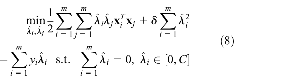
where ${\hat{\lambda }}_i={\lambda }_i^u-{\lambda }_i^l$ .

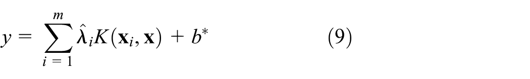
For nonlinear multi-dimensional data, the SVM maps the original data to a higher-dimensional space by kernel function $K({\mathbf{x}}_i,\mathbf{x})=<\varphi ({\mathbf{x}}_i)·\varphi (\mathbf{x})>$ . ²⁹ In this way, the separable hyperplane is identified by transforming the nonlinear problem into the linear one, as shown in equation (9)

$$y=\sum _{i=1}^m{\hat{\lambda }}_{i}K({\mathbf{x}}_i,\mathbf{x})+b^{*}$$

(9)

Quadratic programming problem solution based on the sequential minimum optimization

The sequential minimum optimization (SMO) method ³⁰ is applied to handle the quadratic programming problem in equation (6) to determine $\mathbf{w}$ and $b$ . To facilitate the solution, make the following transformation

$$\{\begin{array}{c}{\hat{\lambda }}_i={\hat{\lambda }}_i^k+d_i\hfill \\ \multicolumn{1}{c}{{\hat{\lambda }}_j={\hat{\lambda }}_j^k+d_j}\end{array},d_i=-d_j$$

(10)

Then, substituting equation (10) into equation (8), the optimal problem with two variables is reduced, as shown in equation (11)

$$\begin{array}{l}\underset{{\widehat{\lambda }}_i,{\widehat{\lambda }}_j}{\min }\frac{1}{2}\left({K^{\prime }}_{ii}-2{K^{\prime }}_{ij}+{K^{\prime }}_{jj}+\delta \right)d_j^2\\ +[\nabla F{({\widehat{\lambda }}^k)}_j-\nabla F{({\widehat{\lambda }}^k)}_i]d_j\\ \mathrm{s}.\mathrm{t}.L\le d_j\le H\end{array}$$

(11)

where

$$\begin{array}{c}\left[\begin{array}{c}\nabla F{\left({\hat{\lambda }}^k\right)}_i\hfill \\ \multicolumn{1}{c}{\nabla F{\left({\hat{\lambda }}^k\right)}_j}\end{array}\right]=\left[\begin{array}{cc}{K\prime }_{\mathrm{ii}}\hfill & {K\prime }_{\mathrm{ij}}\hfill \\ \multicolumn{1}{c}{{K\prime }_{\mathrm{ji}}}& {K\prime }_{\mathrm{jj}}\hfill \end{array}\right]\left[\begin{array}{c}{\hat{\lambda }}_i^k\hfill \\ \multicolumn{1}{c}{{\hat{\lambda }}_j^k}\end{array}\right]+\left[\begin{array}{c}{y}_i\hfill \\ \multicolumn{1}{c}{y_j}\end{array}\right]+\delta \left[\begin{array}{c}{d}_i\hfill \\ \multicolumn{1}{c}{d_j}\end{array}\right]\hfill \\ \{\begin{array}{c}L=max({\hat{\lambda }}_i-C,-C-{\hat{\lambda }}_j)\hfill \\ \multicolumn{1}{c}{H=min({\hat{\lambda }}_i+C,C-{\hat{\lambda }}_j)}\end{array}\hfill \end{array}$$

and k represents the kth iteration.

Suppose that the optimal parameters $\hat{\lambda }{\prime }_i,i=1,2,\dots ,m$ and $b\prime$ are obtained, the regression function is given by equation (12)

$$y=\sum _{i=1}^m{\hat{\lambda }\prime }_{i}K({\mathbf{x}}_i,\mathbf{x})+b\prime$$

(12)

Commonly, linear, polynomial, and Gaussian functions are used as kernel functions. ³¹ The linear kernel function has the advantages of simplicity and strong interpretability, but it can only be used to solve linearly separable problems. Polynomial kernel functions can be used to solve nonlinear problems, but many hyperparameters are generally used in the case of small power. The Gaussian kernel could map the raw data into the high dimensionality space and only need to tune two hyperparameters. Thus, in this study, the Gaussian function is used as kernel function, as shown in equation (13)

$$K({\mathbf{x}}_i,\mathbf{x})=\exp (-\gamma {\Vert {\mathbf{x}}_i-\mathbf{x}\Vert }^2)$$

(13)

where $\gamma$ means the Gaussian coefficient. The prediction performance is achieved by tuning the values of $\gamma$ and $C$ by the cross-validation process at the calibration stage. The pseudocode of the WAS prediction algorithm is expressed in Table 1.

Table 1.

The WAS prediction algorithm.

INPUT: Choose training set randomly (80% data set) Procedure: 1: Data preprocessing 2: Selection of the kernel function and give the range of hyperparameters C and $\gamma$ 3: For $C=C_{min}:C_{max}:\mathrm{\Delta }C$ : 4: For $\gamma ={\gamma }_{min}:{\gamma }_{max}:\mathrm{\Delta }\gamma$ : 5. Initialization variables: d, blow and bup, ${\hat{\lambda }}^0=0$ , set k = 0 6. while (false) do 7. ${\hat{\lambda }}_i,{\hat{\lambda }}_j$  ← select parameters to optimize 8. Solve the equation (11) 9. Update ${\hat{\lambda }}_i^k,{\hat{\lambda }}_j^k$  ←  ${\hat{\lambda }}_i^{k+1},{\hat{\lambda }}_j^{k+1}$ 10. $k\leftarrow k+1$ 11. End while, Obtained $\hat{\lambda },b$ 12: Establish regression function (12) 13: Calculate loss value 14: IF $\mathrm{error}(C,\gamma )<\mathrm{error}(C_{\mathrm{new}},{\gamma }_{\mathrm{new}})$ 15: ELSE IF $(C,\gamma )\leftarrow (C_{\mathrm{new}},{\gamma }_{\mathrm{new}})$ 16: ENDFOR 17: ENDFOR 18: Obtain optimal C and $\gamma$ corresponding to min{error} 19: Verified model performance in test data set (20% data set) OUTPUT: target value $y$

Results

Exploratory data analysis

The descriptive statistical results of the WAS are visible in Table 2. As shown in Table 2, the mean WAS value for the entire data set is 64.4%. For other soil parameters, the clay, sand, silt, and OC have mean values of 16.94, 27.07, 55.99, and 0.87. The mean value of DP is 2.48 g/cm³. The highest mean value of WAS is grass soil (69.04%) for different land uses, while the lowest is found in crop soil (61.80%). For the rest of the soil properties, the cultivated soil shows the highest amount of clay and silt, while the highest level of sand is observed on the bare land. OC is different in various land uses, and the increase of the mean values in the order bare < crop < grass. The change of DP is insignificant in all land uses.

Table 2.

Descriptive statistics for WAS in various land uses.

Land use	N		Clay	Silt	Sand	DP	OC	WAS
			%	%	%	g/cm	%	%
Bare	56	Minimum	6.68	6.98	36.2	2.24	0.37	33.73
		Maximum	35.22	42.03	79.54	2.62	1.10	95.92
		Mean	16.74	24.79	58.57	2.50	0.77	64.00
Crop	47	Minimum	7.36	13.44	34.2	2.26	0.1	25.14
		Maximum	25.71	42.94	73.68	2.65	1.95	91.86
		Mean	17.41	28.96	53.63	2.48	0.87	61.80
Grass	31	Minimum	9.14	13.60	36.29	2.21	0.49	43.16
		Maximum	27.97	48.01	74.15	2.55	2.05	93.65
		Mean	16.59	28.31	55.1	2.44	1.04	69.04
All soil	134	Minimum	6.68	6.98	34.20	2.21	0.1	25.14
		Maximum	35.22	48.01	79.54	2.65	2.05	95.92
		Mean	16.94	27.07	55.99	2.48	0.87	64.40

DP: particle density; OC: organic carbon; WAS: wet aggregate stability.

Pearson’s correlation coefficients among the soil properties in the total data set and in the different land-use patterns are visible in Figure 1. In the various land-use types, the OC is positively correlated with the WAS, while a negative correlation is presented between the DP and the WAS, and all the OC correlations are more significant than 0.4. A negative relationship is observed between clay and WAS (except for grass). The silt is associated with the WAS positively in all data set, bare and grass land uses, while it is uncorrelated with the WAS in the crop soil. The sand is negatively correlated with WAS in grassland and has weak positive correlations in cropland, but there are no correlations in all data sets and bare land.

Figure 1.

The correlation coefficients among soil properties and WAS for various land uses: (a) all data sets, (b) crop data set, (c) bare data set, (d) grass data set.

The WAS prediction based on SVM

A couple of standard statistical indices are applied, including coefficient of determination (R²) and RMSE, to evaluate the performance. In this work, the parameters C and γ are changed, respectively, from 5 to 25 and 0.01 to 0.50 by an increment of 1 and 0.01. Then, the optimal hyperparameters are determined by the Grid-search approach. Subsequently, the validation is applied to obtain the best parameters for WAS prediction by considering R². Figure 2 displays the result of cross-validation in a three-dimensional (3D) space. As indicated in Figure 2, the minimum value of the cross-validation RMSE is 0.6536, and the corresponding parameters of C and γ are 5 and 0.5. Moreover, the optimal result of cross-validation R² appears to check the hyperparameters’ effect. It is shown that SVM model has the optimal parameters C = 5 and γ = 0.5.

Figure 2.

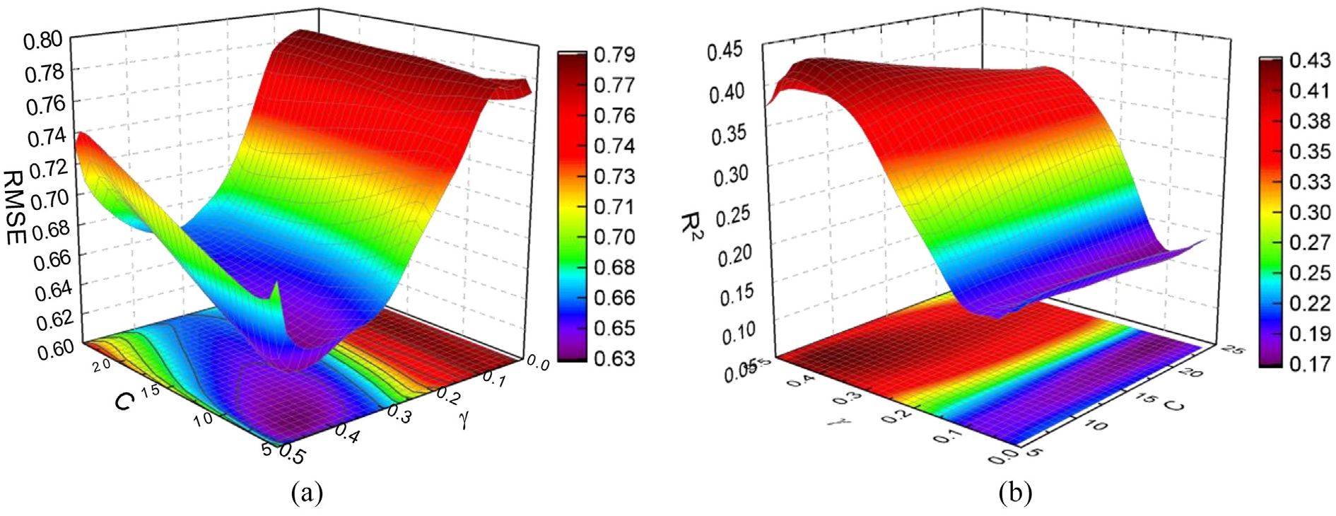
3D plot of RMSE and R² versus C and γ: (a) RMSE versus C and γ, (b) R² versus C and γ.

Subsequently, SVM model is developed by the optimal hyperparameters. The WAS prediction is compared to the actual value to evaluate the performance of the SVM model, as shown in Figure 3. As indicated, the SVM-based model performs well in the training phase (R² = 0.776, RMSE = 7.50) and the testing phase (R² = 0.763, RMSE = 6.81). It is obvious that the SVM model has proper generalization performance in estimating WAS.

Figure 3.

Comparison between actual and predicted WAS from SVM (top) scatter plot and (bottom) samplewise (training: 80% and testing: 20%): (a) SVM-train, (b) SVM-test, and (c) comparison of the predicted and actual WAS.

The WAS prediction based on ANN

In this work, the ANN algorithm is recommended as a reference to evaluate the performance of SVM for WAS prediction. The “relu” function is used as an activation function and an “adam” solver for optimizing weight and bias to generate the ANN model. Then, the ANN model is obtained by adjusting the hidden layer and the number of neurons in each layer. The prediction results in the training and testing phases are illustrated in Figure 4. The ANN has value of R² = 0.664, RMSE = 8.16 in the training stage and R² = 0.665, RMSE = 7.09 in the testing stage. The results indicate that SVM has the edge over ANN in estimating WAS for multiple land-use types.

Figure 4.

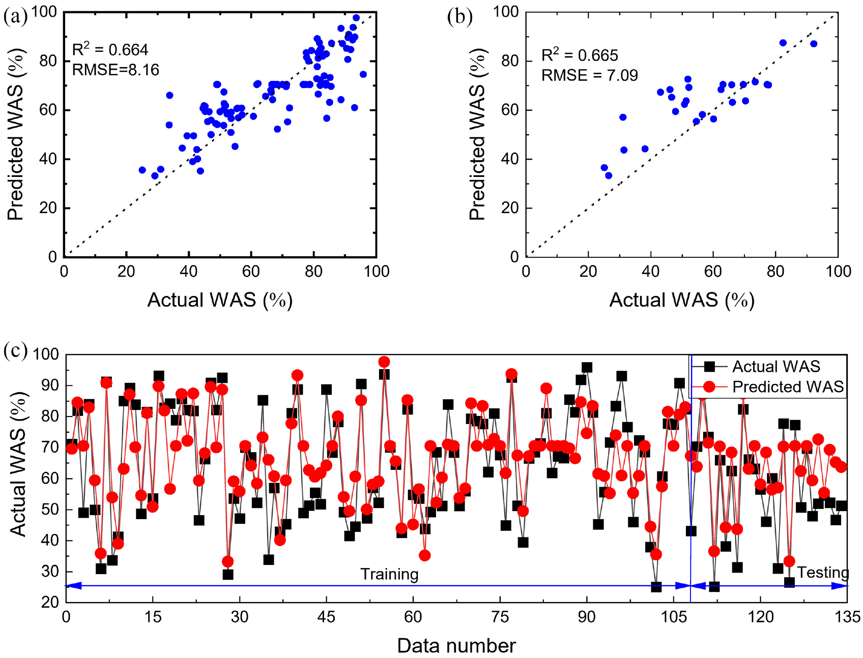
Comparison between actual and predicted WAS from ANN (top) scatter plot and (bottom) samplewise (training: 80% and testing: 20%): (a) ANN-train, (b) ANN-test, and (c) comparison of the predicted and actual WAS.

Comparison with other aggregate stability methods on training and testing data

To evaluate the performance of the proposed method, the SVM model is compared with the existing methods proposed in Usta et al., ¹⁶ Zeraatpisheh et al., ¹⁷ and Ye et al. ³² First, the training data set is predicted. The R² and RMSE values of four methods are calculated. The results are shown in Table 3.

Table 3.

Comparing the performance with existing methods on training data.

Methods	RMSE	R 2
The proposed method	7.5	0.776
Usta et al. 16	12.86	0.53
Zeraatpisheh et al. 17	14.82	0.37
Ye et al. 32	12.66	0.55

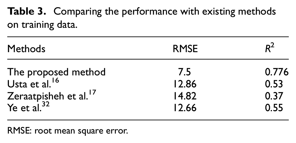
RMSE: root mean square error.

As shown in Table 3, when comparing to Usta et al., ¹⁶ Zeraatpisheh et al., ¹⁷ and Ye et al. ³² , the SVM model provides higher accurate estimation, which reduces the RMSE by 5.36, 7.32, and 5.16, and increases the R² by 0.246, 0.406, and 0.226, respectively. Then, the testing data set is predicted by four methods, and the values of R² and RMSE is listed in Table 4.

Table 4.

Comparing the performance with existing methods on testing data.

Methods	RMSE	R 2
The proposed method	6.81	0.763
Usta et al. 16	13.65	0.48
Zeraatpisheh et al. 17	15.82	0.28
Ye et al. 32	13.38	0.49

RMSE: root mean square error.

For the testing data set, the SVM increases the R² value by 0.283, 0.483, and 0.273, respectively, and the RMSE value decreases 6.84, 9.01, and 6.57, respectively. The comparison illustrates that it has higher performance on the WAS estimation based on SVM.

Analysis of influencing factors

The relative importance (RI) of features is assessed using the SVM model with the sensitivity analysis. The RI is shown in equation (14)

$$\mathrm{RI}\%=\frac{R_{\mathrm{Ommit}}^2}{R_{\mathrm{All}}^2}\times \%$$

(14)

where R²_Ommit is the determination coefficient by omitting a variable, and R²_All is the determination coefficient of all variables.

As shown in Figure 5, OC is the most influential variable, accounting for 33.17% of the variations in the WAS. As the second and third predominant factors, silt and clay provide 21.47% and 19.08% contribution for WAS, which shows the role of micro-particles in soil aggregates, followed by DP (16.46%). By contrast, sand (9.81%) is not critical for WAS.

Figure 5.

Relative importance of features.

Significant properties (OC, silt, and clay) are extracted from Pearson’s correlation and the RI analysis. In this work, the WAS is statistically positively and inversely correlated with OC and DP, respectively, which is in line with other experts.^33,34 Although A Usta et al. ¹⁶ and C Gomez et al. ⁸ observe that WAS increased with clay content, unusual results are offered in the crop, bare, and entire data categories in this research. These results indicate that OC more strongly controls the soil aggregate than the clay and that the WAS is negatively affected by the clay content.^34,35 For the whole data, the low range of clay content could result in the different behavior of the soils; moreover, the different behavior in crop and bare areas might be due to the change in the mineralogy of the clay fraction. In a relatively dry soil environment, the carbonate component of clay harmfully influences soil stability. ³⁶

Despite a low range of OC content in soils, the result shows that OC is the most significant governing property to estimate WAS. OC is the main cementation factor in forming stable aggregates, which forms organo-mineral assemblages with other substances. ³⁷ The application of OC has beneficial impacts on improving soil structure, soil fertility, and reducing surface crusts, which is conducive to plant growth.^34,38 Furthermore, the application of organic carbon is easier to achieve than altering the texture of the soil in large areas.

In addition to soil properties, the remarkable effect of land use and management in WAS can be observed in Table 2. As evident in the table, the WAS differs in various land uses and decreases in the order of grass > bare > crop. ³⁹ There are abundant plant roots in grasslands, a higher abundance of earthworms, and more robust microorganism activity, promoting soil stability. ⁴⁰ By contrast, the tillage destructs the soil structure and reduces biological activity such as earthworm abundance and microbial population.^41,42 Consequently, the average WAS value of the crop soil is lower than that of bare soil. This finding is in line with the observations of S An et al. ⁴³ In general, WAS needs to be improved by increasing vegetation and reducing human disturbance.

Conclusion

This work uses SVM to develop the estimation model for WAS in multiuse soils. The existing models are applied to the WAS data set and compared with the proposed method. The result shows that SVM has the highest performance in predicting WAS with readily measured parameters. Furthermore, WAS is affected by varying parameters and management models. Although the importance of soil parameters is different in various land uses, OC is the most significant factor for predicting WAS. Owing to the broader range of soil components and land uses, the modeling of WAS could be applied to evaluate soil quality in the area short of soil aggregate determination. Our work could be feasible and effective in employing SVM-based model to determine WAS for multiuse soils. In the future, we will establish a larger-scale data set to verify the method comprehensively.