Sage Journals: Discover world-class research

Abstract

To improve the reliability of vehicle state parameter estimation, a vehicle state fusion estimation method based on dichotomy is proposed. An extended Kalman filter algorithm is designed based on the vehicle 3 degrees of freedom dynamic model. Meanwhile, considering the influence of dynamic model and sensor noise and its coefficient selection on the estimation results, a radial basis function neural network estimation algorithm is designed. To further improve the reliability of the estimation algorithm, a method of estimation algorithm fusion is proposed based on the idea of mutual compensation between model- and data-driven estimation algorithms. The weights of the estimation results of different algorithms are assigned through the dichotomy. The redundancy and fusion of estimation algorithms can improve estimation performance. The effectiveness of the fusion method is verified by the co-simulation of MATLAB/Simulink and CarSim, and the real vehicle test. The results show that the change trend of the estimation result is consistent with the actual state parameters change trend, and the estimation accuracy after algorithm fusion is significantly improved compared to a single extended Kalman filter or radial basis function.

Keywords

Vehicle state estimation fusion algorithm radial basis function neural network extended Kalman filter dichotomy

Introduction

Active safety control plays an important role in reducing the incidence of accidents, these systems, such as electronic stability program,^1,2 roll stability control,^3,4 and electric brake-force distribution,^5,6 are related to lateral and longitudinal dynamics. All these control systems can significantly improve the stability control of vehicles, which is by judging the driving environment in advance and accurately intervening in driving. However, the control systems need the many vehicle parameters to participate, among which the side slip, yaw rate and longitudinal speed are difficult to be obtained directly. Therefore, researchers combined the algorithm with the existing sensors on the vehicle to obtain the estimation values of these state parameters that are difficult to be obtained directly.

The commonly used vehicle state parameter estimation methods include Kalman filter (KF) and its improved algorithms,^7–17 neural network estimation algorithms,^18–20 and other related estimation algorithms.^21–27 However, single estimation algorithms have their own limitations, such as the uncertainty of mathematical model parameters, noise parameters, and the coverage of training samples, which will affect the estimation results and may lead to the sudden divergence of estimation accuracy. Therefore, for the problems about the single estimation algorithm, researchers integrate different estimation theories to improve the performance of the whole estimation system through the redundancy and fusion of the algorithm. In the study of fusion estimation algorithms, W Wenkang et al.²⁸ use the interacting multiple model method to realize the fusion of two square root cubature KF with different mathematical models. G Liu and LQ Jin²⁹ use the interacting multiple model method to combine the cubature KF with different mathematical models to estimate the side slip angle and wheel lateral force. T Chen et al.³⁰ use the weighted iterative fusion method to fuse the strong tracking filter with the ridge estimation algorithm to obtain the longitudinal and lateral vehicle speeds, and the side slip angle. X Li et al.³¹ use the adaptive federated fusion algorithm to fuse the adaptive auxiliary filter and the extended Kalman filter (EKF) to estimate the side slip angle and yaw rate. A fusion method proposed by W Liu et al.,¹² which combines the minimum model error algorithm with the EKF algorithm to estimate the side slip angle. BL Gao et al.³² use the dual KF fusion technology to fuse the results estimated by simplified tire magic formula and wheel dynamic formula, which can realize the estimation of road adhesion coefficient. However, these above-mentioned fusion algorithms need to rely on the construction of mathematical model, which make the structure of the fusion algorithm complex and large amount of calculation. To solve this problem, a hybrid-driven estimator based on dichotomy is proposed by combining EKF algorithm based on model driven and radial basis function (RBF) neural network algorithm based on data-driven.

In this article, an EKF algorithm based on vehicle dynamics model is designed. Through the state space equation and observation equation, it can establish the mapping relationship between system input and estimated object. According to this mapping relationship, an RBF neural network estimator without dynamic modeling is designed. A KF algorithm is designed based on 2 degrees of freedom (2-DOF) dynamic model, and is used to obtain estimation values of the side slip angle and yaw rate, which are used as reference values (RVs). Meanwhile, the RV of longitudinal speed is obtained by calculation formula. The weighted fusion of vehicle state estimation results is realized using the dichotomy method, which distributes different weights to outcome of different estimation algorithms judged by error between different estimation values and RVs. This fusion method can suppress the decline of accuracy when a single algorithm estimates different targets, and ensures the reliability of the estimation system and the universality of the fusion method.

The rest of this article is organized as follows. In the “Vehicle dynamic model” section, the 2-DOF and 3-DOF vehicle dynamic models have been established. The “Proposed estimator of vehicle state parallel estimation based on multi-source fusion” section introduces the components of the new fusion estimation method by dichotomy. In addition, the analysis and discussion of the simulation and real vehicle experimental results will be shown in the “Results and discussion” and the “Real vehicle test” sections, respectively. Finally, the conclusion and summary are given in the “Conclusion” section.

Vehicle dynamic model

2-DOF vehicle dynamic model

The KF will be used in this article. Therefore, a 2-DOF vehicle dynamic model is established,³³ as shown in equation (1)

\begin{matrix} {\overset{\cdot}{ω}}_{r} = \frac{a^{2} k_{1} + b^{2} k_{2}}{I_{z} V_{x}} ω_{r} + \frac{a k_{1} - b k_{2}}{I_{z}} β - \frac{a k_{1}}{I_{z}} δ \\ \overset{\cdot}{β} = (\frac{a k_{1} - b k_{2}}{{mV}_{x}^{2}} - 1) ω_{r} + \frac{k_{1} + k_{2}}{m V_{x}} β - \frac{k_{1}}{m V_{x}} δ \end{matrix}

(1)

where ω_r represents yaw rate, a represents the distance between centroid and front axle, b represents the distance between centroid and rear axle, k₁ and k₂ represent the cornering stiffness of the front and rear axles, respectively, V_x represents longitudinal speed, I_z represents moment of inertia, δ represents the steering angle of front wheel, and β represents side slip angle.

Meanwhile, 2-DOF state function and observation function can be obtained

\begin{matrix} \overset{\cdot}{x} = A x + B u \\ y = C x + D u \end{matrix}

(2)

Among them

\begin{matrix} \overset{\cdot}{x} = [\begin{matrix} {\overset{\cdot}{ω}}_{r} \\ \overset{\cdot}{β} \end{matrix}] A = [\begin{matrix} a_{11} & a_{12} \\ a_{21} & a_{22} \end{matrix}] B = [\begin{matrix} b_{11} \\ b_{12} \end{matrix}] \\ y = [\begin{matrix} ω_{r} \\ β \end{matrix}] C = [\begin{matrix} 1 & 0 \\ 0 & 1 \end{matrix}] D = [\begin{matrix} 0 \\ 0 \end{matrix}] u = δ \end{matrix}

where

\begin{array}{l} a_{11} = \frac{a^{2} k_{1} + b^{2} k_{2}}{I_{z} V_{x}} a_{12} = \frac{a k_{1} - b k_{2}}{I_{z}} \\ a_{21} = \frac{a k_{1} - b k_{2}}{m V_{x}^{2}} - 1 a_{22} = \frac{k_{1} + k_{2}}{m V_{x}} \\ b_{11} = - \frac{a k_{1}}{I_{z}} b_{21} = - \frac{k_{1}}{m V_{x}} \end{array}

3-DOF vehicle dynamic model

Based on the 2-DOF dynamic model, longitudinal speed is added as a DOF. The 3-DOF vehicle dynamic model is shown in Figure 1.

Figure 1.

3-DOF vehicle dynamics model considering longitudinal speed.

In Figure 1, F_y1 and F_y2 represent the lateral force of the ground to the front and rear wheels, respectively, V_y represents the lateral speed, and α₁ and α₂ represent the side slip angle of the front and rear wheels, respectively.

The 3-DOF vehicle dynamic model is established,³⁴ as shown in equation (3)

\begin{matrix} {\overset{\cdot}{ω}}_{r} = \frac{a^{2} k_{1} + b^{2} k_{2}}{I_{z} V_{x}} ω_{r} + \frac{a k_{1} - b k_{2}}{I_{z}} β - \frac{a k_{1}}{I_{z}} δ \\ \overset{\cdot}{β} = (\frac{a k_{1} - b k_{2}}{{mV}_{x}^{2}} - 1) ω_{r} + \frac{k_{1} + k_{2}}{m V_{x}} β - \frac{k_{1}}{m V_{x}} δ \\ {\overset{\cdot}{V}}_{x} = V_{x} β ω_{r} + a_{x} \end{matrix}

(3)

where a_x represents the longitudinal acceleration.

The state function is

\begin{matrix} [\begin{matrix} {\overset{\cdot}{ω}}_{r} \\ \overset{\cdot}{β} \\ {\overset{\cdot}{V}}_{x} \end{matrix}] = [\begin{matrix} \frac{k_{1} a^{2} + k_{2} b^{2}}{I_{z} V_{x}} & \frac{k_{1} a - k_{2} b}{I_{z}} & 0 \\ \frac{k_{1} a - k_{2} b - {mV}_{x}^{2}}{{mV}_{x}^{2}} & \frac{k_{1} + k_{2}}{m V_{x}} & 0 \\ V_{x} β & 0 & 0 \end{matrix}] [\begin{matrix} ω_{r} \\ β \\ V_{x} \end{matrix}] \\ + [\begin{matrix} - \frac{k_{1} a}{I_{z}} & 0 \\ - \frac{k_{1}}{m V_{x}} & 0 \\ 0 & 1 \end{matrix}] [\begin{matrix} δ \\ a_{x} \end{matrix}] \end{matrix}

(4)

where k₁ and k₂ can be represented the form as below³⁵

k_{1} = \frac{(bm a_{y} + I_{z} {\overset{\cdot}{ω}}_{r}) V_{x}}{2 (a + b) (δ V_{x} - V_{y} - a ω_{r})}

k_{2} = \frac{(am a_{y} - I_{z} {\overset{\cdot}{ω}}_{r}) V_{x}}{2 (a + b) (b ω_{r} - V_{y})}

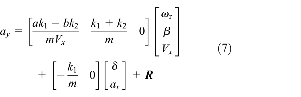
where a_y represents the lateral acceleration.

The observation function is

[a_{y}] = [\frac{a k_{1} - b k_{2}}{m V_{x}} \frac{k_{1} + k_{2}}{m} 0] [\begin{matrix} ω_{r} \\ β \\ V_{x} \end{matrix}] + [- \frac{k_{1}}{m} 0] [\begin{matrix} δ \\ a_{x} \end{matrix}]

(5)

Proposed estimator of vehicle state parallel estimation based on multi-source fusion

This article establishes a new fusion estimation method to estimate the yaw rate, side slip angle, and longitudinal speed. The structure diagram of the proposed fusion estimation method is shown in Figure 2. The proposed fusion method consists of four parts: (1) EKF estimator based on model-driven; (2) the RBF neural network estimator based on data-driven; (3) the RVs are obtained from KF or algebraic formula, which is used as the benchmark value; and (4) the fusion estimation algorithm (FEA) based on dichotomy will assign appropriate weight to the estimation values of the two algorithms, respectively, and then output a new fitted signal.

Figure 2.

Estimator architecture.

Extended KF algorithm

The EKF is to simplify the linearization of the nonlinear state by first-order Taylor expansion, which ignores the higher-order terms for the state function. From the “Vehicle dynamic model” section, the 3-DOF dynamic equation considering the longitudinal speed is obtained. Furthermore, linearize the state equation and observation equation to obtain the linearized model.

Based on equations (4) and (5), functions (6) and (7), including process noise and observation noise, can be obtained

\begin{matrix} [\begin{matrix} {\overset{\cdot}{ω}}_{r} \\ \overset{\cdot}{β} \\ {\overset{\cdot}{V}}_{x} \end{matrix}] = [\begin{matrix} \frac{k_{1} a^{2} + k_{2} b^{2}}{I_{z} V_{x}} & \frac{k_{1} a - k_{2} b}{I_{z}} & 0 \\ \frac{k_{1} a - k_{2} b - {mV}_{x}^{2}}{{mV}_{x}^{2}} & \frac{k_{1} + k_{2}}{m V_{x}} & 0 \\ V_{x} β & 0 & 0 \end{matrix}] [\begin{matrix} ω_{r} \\ β \\ V_{x} \end{matrix}] \\ + [\begin{matrix} - \frac{k_{1} a}{I_{z}} & 0 \\ - \frac{k_{1}}{m V_{x}} & 0 \\ 0 & 1 \end{matrix}] [\begin{matrix} δ \\ a_{x} \end{matrix}] + Q \end{matrix}

(6)

\begin{matrix} a_{y} = [\frac{a k_{1} - b k_{2}}{m V_{x}} \frac{k_{1} + k_{2}}{m} 0] [\begin{matrix} ω_{r} \\ β \\ V_{x} \end{matrix}] \\ + [- \frac{k_{1}}{m} 0] [\begin{matrix} δ \\ a_{x} \end{matrix}] + R \end{matrix}

(7)

The Q matrix is considered as constant and diagonal, whose elements have been calculated considering the square value of the expected maximum variation for each state variable. R is positive definite and it changes during time according to different covariance calculations on a moving window of length equal to 0.01 s.

Q_{i} = \frac{1}{{(x_{i_{max}} - x_{i_{\min}})}^{2}} i = (1, 2, . . ., t)

(8)

Equations (6) and (7) can be written in the following form

\begin{matrix} x (t) = w (x (t), u (t), q (t)) \\ y (t) = z (x (t), r (t)) \end{matrix}

where x (t) represents the state variable of the system, y (t) represents the measurement output, u (t) represents the system input, u (t) = [δ a_x]^T, q (t) represents the system noise, and r (t) represents the measurement noise.

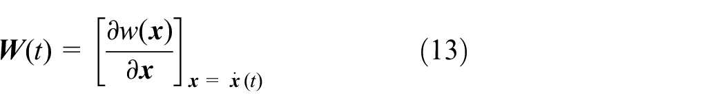
The Jacobian matrix is obtained by partial differentiation of the state equation and the observation equation, respectively, and the Jacobian matrix is shown as below

W (t) = {[\frac{\partial w (x)}{\partial x}]}_{x = \dot{x} (t)}

Z (t) = {[\frac{\partial z (x)}{\partial x}]}_{x = \dot{x} (t)}

γ (t) = e^{W (t) \times Δ t} \approx W (t) \times Δ t + I

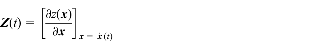
where $Δ t$ represents sample time, W (t) and Z (t) represent the Jacobian matrix of the partial derivatives of the nonlinear functions w( x (t), u (t), ( q (t)) and z( x (t), r (t)) with respect to the state variables, respectively, and $γ (t)$ represents the state transition matrix.

First-order linearized form of the dynamic model can be written as

\begin{matrix} W (t) = \\ [\begin{matrix} \frac{ω_{r} a^{2} + β b^{2}}{I_{z} V_{x}} & \frac{k_{1} a - k_{2} b}{I_{z}} & - \frac{(k_{1} a^{2} + k_{2} b^{2})}{I_{z} V_{x}} ω_{r} \\ \frac{k_{1} a - k_{2} b - m {v_{x}}^{2}}{m {V_{x}}^{2}} & \frac{k_{1} + k_{2}}{m {V_{x}}^{2}} & - \frac{2 ω_{r} (k_{1} a - k_{2} b)}{m {V_{x}}^{3}} - β \frac{(k_{1} + k_{2})}{m {V_{x}}^{2}} + \frac{δ k_{1}}{m {V_{x}}^{2}} \\ V_{x} β & V_{x} ω_{r} & ω_{r} β \end{matrix}] \end{matrix}

(9)

Z (t) = [\begin{matrix} \frac{k_{1} a - k_{2} b}{m V_{x}} \\ \frac{k_{1} + k_{2}}{m} \\ - \frac{k_{1} a - k_{2} b}{m {V_{x}}^{2}} \end{matrix}]

(10)

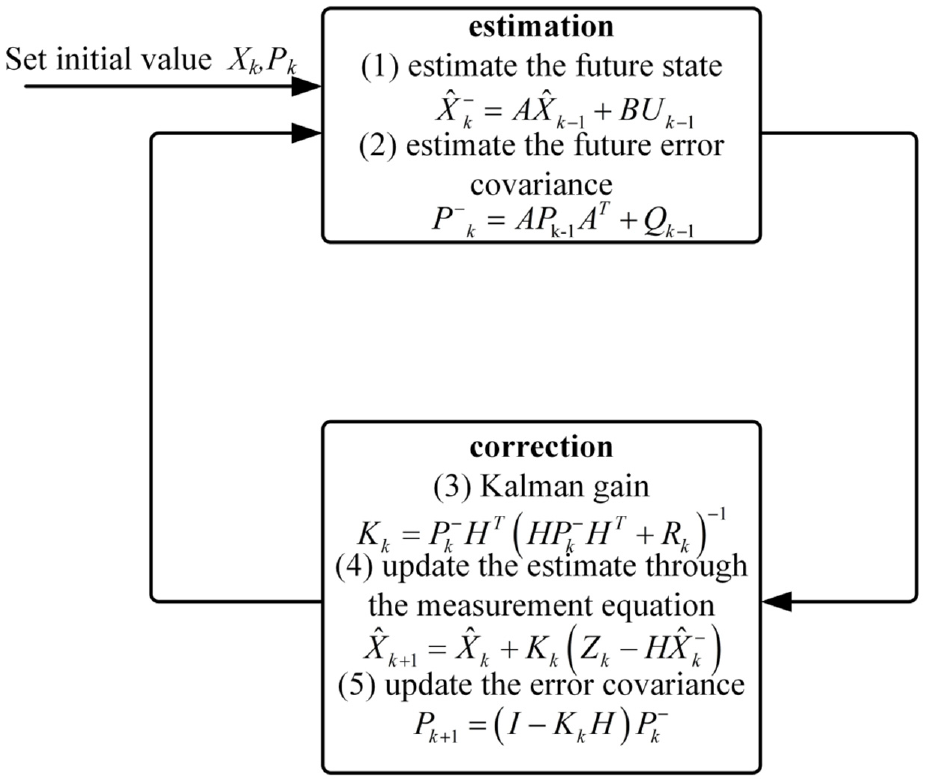
One calculation cycle of EKF is as follows:

Step 1: Initialization initial state x₍₀ ₎, covariance matrix P₀ .

Step 2: State prediction

x (t | t - 1) = w (x (t - 1), u (t - 1), q (t - 1))

(11)

Step 3: Observation prediction

y (t | t - 1) = z (x (t - 1), r (t - 1))

(12)

Step 4: Fig out the first-order linearized expression of the state equation, and solve the state transition matrix W (t)

W (t) = {[\frac{\partial w (x)}{\partial x}]}_{x = \dot{x} (t)}

(13)

Step 5: Fig out the first-order linearized expression of the observation equation, and solve the observation matrix Z (t)

Z (t) = {[\frac{\partial z (x)}{\partial x}]}_{x = \dot{x} (t)}

(14)

Step 6: Fig out the covariance matrix P (t–1|t)

P (t | t - 1) = W (t) P (t - 1 | t - 1) W^{T} (t) + Q

(15)

Step 7: Solve Kalman gain

K (t) = P (t | t - 1) H^{T} (t) (H (t) P (t | t - 1) H^{T} (t) + R)

(16)

Step 8: Status update

x (t) = x (t | t - 1) + K (y (t) - y (t | t - 1))

(17)

Step 9: Covariance update

P (t) = (I - K (t) H (t)) P (t | t - 1)

(18)

Radial basis function neural network algorithm

RBF neural network is an artificial neural network that uses RBFs as activation function. The RBF neural network in this article is used to estimate the vehicle state parameters.

The differential equation (1) of the vehicle 3-DOF dynamic model obtained in the “Vehicle dynamic model” section is transformed into the state function form, as shown in equation (19)

{\hat{x}}_{k} = f (x_{k - 1}, u_{k - 1})

(19)

It can be seen from equation (19) that the change of the system state variable is determined by the system input, and it can be considered that exist a mapping relationship between the state variable and the state input. When steering wheel angle and longitudinal acceleration determined, the equations about yaw rate, side slip angle, and longitudinal speed have unique solutions. There is a specific functional relationship between them, as shown in formulas (20)–(22)

β = f (a_{x}, δ)

(20)

ω_{r} = f (a_{x}, δ)

(21)

V_{x} = f (a_{x}, δ)

(22)

To make the training sample basically cover the driving condition, the set operation conditions are shown in Table 1.

Table 1.

Obtain driving conditions of training samples.

Operating conditions	Speed
Operating conditions	Uniform acceleration (km/h)	Uniform deceleration (km/h)	Variable acceleration (km/h)
Straight driving	20–70	80–30	10–60
Turn driving	20–70	80–30	10–60
Serpentine driving	20–70	80–30	10–60

The training sample is obtained by the co-simulation of CarSim and MATLAB/Simulink. The steering wheel angle and longitudinal acceleration are collected by CarSim as the input of training sample, which corresponding yaw rate, side slip angle, and longitudinal speed are used as the output of training sample. The collected data sets are divided into training samples and test samples. Finally, the trained RBF neural network can be used for state estimation.

As shown in Figure 3, the structure of the RBF in this article contains two layers, a hidden radial basis layer of A¹ neurons and an output-linear layer of A² neurons. To reduce the training time of neural network, the 15,000 groups of data are obtained by interval value processing, and finally, 3000 groups of data are obtained. Based on the Kolmogorov theory, the number of neurons in the hidden layer is set to 5. The RBF neural network estimation methods are introduced by Schwenker et al.³⁶ The related RBF is radf(n) = e^-n2, the purelin represents linear transfer function, and||dist|| is Euclidean distance weight function.

Figure 3.

Radial basis function neural network architecture.

In Figure 3,

N represents number of elements in input vector;

A ¹ represents number of neurons in hidden layer;

A ² represents number of neurons in linear layer;

IZ_1,1 represents input weight matrix;

LZ_2,1 represents linear layer weight;

X represents input sample.

b ₁ and b₂ are neuron thresholds of hidden and linear layers, respectively;

op ¹ represents the results calculated by RBF radf and the function is shown as below

o p^{1} = radf (| | I Z_{1, 1} - X | | b_{1})

op ² represents the results calculated by linear transfer function purelin and the function is shown as below

o p^{2} = purelin (L Z_{2, 1} o p^{1} - b_{2})

The training process of RBF neural network is as follows

1. Calculation error e_j

e_{j} = d_{j} - f (X_{j}) = d_{j} - \sum_{i = 1}^{M} ω_{i} G (X_{j}, T_{i})

(23)

where d_j represents the expected output, f(X_j) represents the network prediction output, X_j represents the input of the jth neuron, T_i represents neuronal center, and ω_i represents connection weight.

2. Calculate the output weight change

\frac{\partial E (n)}{\partial ω_{i} (n)} = - \frac{1}{N} \sum_{j = 1}^{N} e_{j} \exp (\frac{- {‖ X_{j} - T_{i} ‖}^{2}}{2 σ_{i}^{2}})

(24)

Then, use formula (25) to adjust the weight

ω_{i} (n + 1) = ω_{i} (n) - η_{1} \frac{\partial E (n)}{\partial ω_{i} (n)}

(25)

where η₁ represents the learning rate when the weight is adjusted.

3. The central changes of neurons in the hidden layer were calculated

\frac{\partial E (n)}{\partial T_{i} (n)} = - \frac{ω_{1}}{N σ_{i}^{2}} \sum_{j = 1}^{N} e_{j} \exp (\frac{- {‖ X_{j} - T_{i} ‖}^{2}}{2 σ_{i}^{2}}) {(X_{j} - T_{i})}^{2}

(26)

The adjustment center is shown as equation (27)

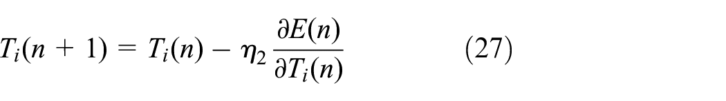
T_{i} (n + 1) = T_{i} (n) - η_{2} \frac{\partial E (n)}{\partial T_{i} (n)}

(27)

where η₂ represents the learning rate when the center change is adjusted.

4. Calculate the change of output weight

\frac{\partial E (n)}{\partial T_{i} (n)} = - \frac{ω_{1}}{N σ_{i}^{3}} \sum_{j = 1}^{N} e_{j} \exp (\frac{- {‖ X_{j} - T_{i} ‖}^{2}}{2 σ_{i}^{2}}) {(X_{j} - T_{i})}^{2}

(28)

Adjust the width is shown as equation (29)

σ_{i} (n + 1) = σ_{i} - η_{3} \frac{\partial E (n)}{\partial T σ_{i} (n)}

(29)

where η₃ represents the learning rate when the center width is adjusted.

5. Calculate the total error value

E = \frac{1}{2 N} \sum_{j = 1}^{N} e_{j}^{2}

(30)

Fusion estimation algorithm

In the “Extended KF algorithm” and the “Radial basis function neural network algorithm” sections, the two kinds of estimation algorithm have been stated clearly. The determination for different estimation algorithm weights will be considered in this section. In this selection, the RV and determination of weights corresponding to different estimation algorithms are included.

The function of the RV is regarded as a benchmark. Therefore, there is no high precision requirement for the prediction result of the RV. It only needs to be consistent with the actual change trend of the estimated object. The KF algorithm based on 2-DOF vehicle dynamic model is used to obtain the yaw rate and side slip angle, and be as benchmark value. The workflow of KF is shown in Figure 4.

Figure 4.

Workflow of KF.

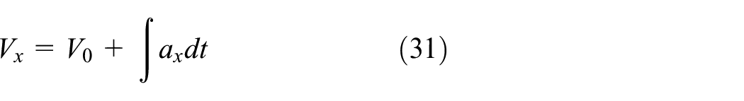
In Figure 4, A represents state transition matrix, B represents system input matrix, H represents observation matrix, Z represents the measurement matrix, X represents the state variable matrix, and U represents the system input matrix.

The formula is applied to the selection of the RV for longitudinal speed as below³⁷

V_{x} = V_{0} + \int a_{x} dt

(31)

When the estimation results of different estimation algorithms have been collected, the dichotomy is used to search for the weight in the FEA. The basis of the selection is at a certain moment, the error 1(e₁) is the error between the estimation value of algorithm 1 and the RV, the error 2(e₂) is the error between the estimation value of algorithm 2 and the RV.

In a certain step k, the proportional relationship between e₁(k) and e₂(k) is determined by dichotomy, which is converted into the form of weight and assigned to different estimation algorithms. The smaller error has a greater weight of the estimation algorithm, and a new estimated signal is fitted finally. The diagram is shown in Figure 5, and the determination of weights can be divided into two cases.

Figure 5.

Diagram of prediction error.

The weight search steps are as follows:

Step 1: Obtaining the target estimation value, RV and obtaining error

\begin{matrix} e_{1} (k) = | x_{REF_L} (k) - {\hat{x}}_{a 1_L} (k) | \\ e_{2} (k) = | x_{REF_L} (k) - {\hat{x}}_{a 2_L} (k) | \\ (L = ω_{r}, β, V_{x}) \end{matrix}

where x_{REF_L} represents the RV, the ${\hat{x}}_{a 1_L}$ represents the estimation value of algorithms 1, the ${\hat{x}}_{a 2_L}$ represents the estimation value of algorithm 2.

Step 2: Searching weigh

{\begin{matrix} A_{k} = lim_{s - r \to d} \frac{| x_{R_L} (k) - {\hat{x}}_{a 1_L} (k) |}{| x_{R_L} (k) - {\hat{x}}_{a 2_L} (k) |} \\ B_{k} = 1 - lim_{s - r \to d} \frac{| x_{R_L} (k) - {\hat{x}}_{a 1_L} (k) |}{| x_{R_L} (k) - {\hat{x}}_{a 2_L} (k) |} \end{matrix}

where d represents the weight precision, and s and r represent weight search range [r, s].

Step 3: output update

y_{L} (k) = A_{k} \cdot {\hat{x}}_{a 2_L} (k) + B_{k} \cdot {\hat{x}}_{a 1_L} (k)

Results and discussion

The experiment was completed by related simulation software and true value output by simulation software. Table 2 shows the relevant parameters of the vehicle model in the simulation software.

Table 2.

Vehicle parameters.

Vehicle configuration parameters	Value
Vehicle weight, m/kg	1229
Distance from centroid to front axle, a/m	1.020
Distance from centroid to rear axle, b/m	1.560
Moment of inertia, I_z/(kg m²)	1536.7
Centroid height, h/m	0.54

Estimated results of side slip angle

The side slip angle experimental results are shown in Figures 6 –8.

Figure 6.

Comparison of estimation value of EKF, RBF, and RV with true value of side slip angle.

Figure 7.

Comparison of estimation value of FEA with true value of side slip angle.

Figure 8.

Relative error with non-zero true value of side slip angle.

In the figure, the beta of ekf, the beta of rbf, and the beta of opt is the side slip angle estimated by the EKF, RBF algorithms, and FEA, respectively. Meanwhile, the beta of true is true value of side slip angle obtained by CarSim, and beta of ref is RV of side slip angle.

It can be seen from Figure 6 that the beta of ref can well reflect the change trend of the actual side slip angle. At the same time, the estimation values of the side slip angle obtained by EKF and RBF have a small deviation from the true value, and the average of absolute error between them and the true value is 0.1176 and 0.1512, respectively. In Figure 7, the estimation result of FEA is consistent with the true value, and the average of absolute error of FEA is 0.0802. The estimation accuracy of FEA is 31.80% higher than EKF and 46.95% higher than RBF. Therefore, the estimation result of FEA is better than the estimation result of a single estimation algorithm. The relative error result can be seen from Figure 8, and the relative error of the estimation value of FEA is within 13%.

Estimated results of yaw rate

The yaw rate experimental results are shown in Figures 9 –11.

Figure 9.

Comparison of estimation value of EKF, RBF, and FEA with true value of yaw rate.

Figure 10.

Comparison of estimation value of FEA with true value of yaw rate.

Figure 11.

Relative error with non-zero true value of yaw rate.

In the figure, ω of ekf, ω of rbf, and ω of opt are the yaw rate estimated by the EKF, RBF algorithms, and FEA, respectively. Meanwhile, the ω of true is true value of yaw rate obtained by CarSim, and ω of ref is RV of yaw rate.

It can be seen from Figure 9 that the ω of ref can well reflect the change trend of the actual yaw rate. At the same time, the results estimated by the RBF algorithm and the EKF algorithm are quite different. The result of the EKF began to shift in the third second, its accuracy gradually reduced until the eighth second. On the contrary, the estimation result of the yaw rate by the RBF is close to the true value except for the slight fluctuation in the first 2.5 s. The estimation result of FEA can be seen from Figure 10 that the estimated accuracy has a short drop in 3.1–3.5 and 5.3–6.5 s, but it returns to normal immediately. Except for two short fluctuations, the average absolute errors of FEA, EKF, and RBF are 0.5825, 9.3653, and 0.5914, respectively. The estimation accuracy of FEA is 93.37% higher than EKF and 1.5% higher than RBF. Therefore, the estimation result of FEA is better than that of the single estimation algorithm. The relative error with non-zero true value can be seen from Figure 11, and the relative error of the estimation value of FEA is within 14%.

Estimated results of longitudinal speed

The longitudinal speed experimental results are shown in Figure 12.

Figure 12.

(a) Comparison of EKF, RBF, and RV with true value, (b) comparison between estimation value of FEA and true value, (c) comparison of absolute error of EKF and RBF with FEA, and (d) relative error of longitudinal speed estimation value of FEA.

In the figure, the Vx of ekf, Vx of rbf, and Vx of opt are the longitudinal speed estimated by the EKF, RBF, and FEA, respectively. Meanwhile, the Vx of true is true value of longitudinal speed obtained by CarSim, and Vx of ref is RV of longitudinal speed.

It can be seen from Figure 12(a) that the Vx of ref can well reflect the change trend of the actual longitudinal speed. At the same time, the accuracy of longitudinal speed estimation results obtained by EKF is lower, but the estimation value change trend is consistent with the true value. On the contrary, the estimation result of the longitudinal speed by the RBF is close to the true value except for the two fluctuations in the 0–2.5 and 9.3–10 s. It can be seen from Figure 12(b) that under the weight distribution of the FEA, the final estimation value can maintain high consistency with the true value of longitudinal speed. As shown in Figure 12(c), the estimation results of EKF, RBF, and FEA are evaluated by the average value of absolute error, which are 9.57, 7.332, and 1.96, respectively. Therefore, the estimated accuracy of FEA is 79.5% higher than EKF, and 73.2% higher than RBF. It can be seen from the comparison that the estimation result after the FEA is better than the estimation result of a single estimation algorithm, and the relative error of the estimation value of FEA is still within 12% in Figure 12(d).

Real vehicle test

Through the co-simulation results of CarSim and MATLAB/Simulink in the “Results and discussion” section, the feasibility of the vehicle state fusion estimation method based on dichotomy is preliminarily verified. In this section, the vehicle state fusion estimation method is further verified through the real vehicle test. However, due to the limitation of equipment acquisition capacity, the true value of side slip angle cannot be collected.

In this section, under the driving condition of double lane change, the yaw rate and longitudinal speed are estimated using the FEA, and compared with the true values collected by the equipment. The real vehicle test workflow is shown in Figure 13, and the ω_r_{_exp} and V_x_{_exp} represent the yaw rate and longitudinal speed obtained by acquisition equipment, respectively.

Figure 13.

Real vehicle test workflow.

The hardware equipment involved in the real vehicle test includes: real vehicle, CANoe analyzer, gyroscope, and GPS antenna. Through CANoe analyzer, gyroscope, and GPS antenna, the state parameters, which is include front wheel angle, yaw rate, longitudinal speed, longitudinal acceleration, and lateral acceleration during driving, are collected. The collected data are divided into two parts: the one part is used for the training of RBF neural network and the other part of the data is used as the input of the estimation system for the estimation of yaw rate and longitudinal vehicle speed. Finally, the collected yaw rate and longitudinal vehicle speed are compared with the estimation results to verify the proposed fusion estimation method.

The signal curves of the longitudinal acceleration, lateral acceleration, and steering wheel angle are shown in Figures 14 –16.

Figure 14.

Longitudinal acceleration.

Figure 15.

Lateral acceleration.

Figure 16.

Front wheel steer angle.

The experiment results are shown in Figures 17 –20, and the ω/V_x of EKF, ω/V_x of RBF, and ω/V_x of REF represent the outcome obtained by EKF, RBF, and RV, respectively. The ω/V_x of opt represents the estimation result obtained by FEA and the ω/V_x of mv represents the measured value.

Figure 17.

The yaw rate obtained by different methods.

Figure 18.

The final estimation value and the experimental value of yaw rate.

Figure 19.

The longitudinal speed obtained by different methods.

Figure 20.

The final estimation value and the experimental value of longitudinal speed.

The ω of REF in Figure 17 can reflect the change trend of the actual yaw rate. At the same time, the estimation values of EKF and RBF are similar, but their estimation results of yaw rate are different at 2.2–2.8 and 5.6–6 s, respectively. Finally, the estimation values of EKF and RBF are fused by FEA to obtain the final estimation value, as shown in the ω of opt of Figure 18.

The Vx of REF in Figure 19 can reflect the change trend of the actual longitudinal speed. At the same time, the estimation values of EKF and RBF are generally similar, but their estimation results of longitudinal speed are different at 0–0.23, 2–2.85, and 3.8–5.1 s, respectively. Finally, the estimation values of EKF and RBF are fused by FEA to obtain the final estimation value, as shown in the Vx of opt of Figure 20.

It can be seen from Figures 18 and 20 that the estimation result after FEA maintains high consistency with the true value. To further verify the superiority of the fusion estimation method proposed in this article, the root mean square (RMS) error between the estimation value and the true value is used to evaluate the estimation performance, which can be expressed as

e_{RMS} = \sqrt{\frac{1}{n} \sum_{i = 1}^{n} {({\hat{y}}_{i} - y_{i})}^{2}}

(32)

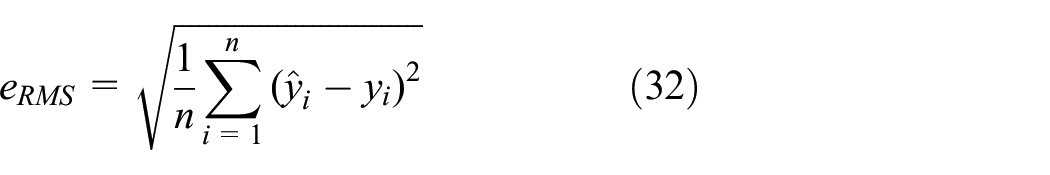
where ${\hat{y}}_{i}$ represents the final estimation value and $y_{i}$ represents the true value.

The e_RMS can be seen in Table 3, it can be found that the RMS errors of yaw rate and longitudinal speed estimated based on FEA is less than EKF and RBF, indicating that FEA can better suppress the error of single algorithm and improve the estimation accuracy. Compared with the RMS of EKF and RBF, the FEA is increased by 57.2% and 45.1%, respectively, in estimation of yaw rate, and compared with the 0.8135 of RMS of other FEAs,³⁸ the FEA is increased by 71.2%. Compared with the RMS of EKF and RBF, the FEA is increased by 96.2% and 83.4%, respectively, in estimation of longitudinal speed, and compared with the 0.6876 of RMS of other FEAs,³⁹ the FEA is increased by 80.4%.

Table 3.

Root mean square error comparison.

State parameters	Estimated algorithms	e_RMS
Yaw rate	EKF	0.5459
	RBF	0.4257
	FEA	0.2336
Longitudinal speed	EKF	3.6023
	RBF	0.8161
	FEA	0.1349

EKF: extended Kalman filter; RBF: radial basis function; FEA: fusion estimation algorithm.

Conclusion

The EKF estimator is designed based on the vehicle dynamic model. At the same time, the operating conditions that the estimation results are inaccurate or unable to be estimated when the measurement noise is non-Gaussian noise or the observation sensor is disabled are considered. An RBF neural network estimator is designed, which does not depend on the dynamic model and is not affected by the observation sensor.

The vehicle dynamics model estimator is combined with the non-vehicle dynamics model estimator, and the dichotomy is used to find the weights of different estimation results, which can realize the fusion of vehicle state estimation algorithms and improve the performance of the estimation system.

Through the co-simulation, the fusion method is verified. The results based on real vehicle test show that the proposed fusion method can maintain high consistency between the final estimation value and the true value, and accurately reflect the change trend of vehicle state parameters.

Footnotes

Handling Editor: Yanjiao Chen

Declaration of conflicting interests

The author(s) declared no potential conflicts of interest with respect to the research, authorship, and/or publication of this article.

Funding

The author(s) disclosed receipt of the following financial support for the research, authorship, and/or publication of this article: After examination, this paper is supported by the Scientific Research Foundation of Fujian University of Technology (grant no. GY-Z19010).

ORCID iD

Xinye Liu

References

Fan

Zhao

. Vehicle dynamics modeling and electronic stability program/active front steering sliding mode integrated control. Asian J Control 2019; 21(5): 2364–2377.

Wibowo

Amirulloh

Hanafi

, et al. Robust control for electronic stability program (ESP) on four wheel vehicle prototype. In: Proceedings of the 2017 international electronics symposium on engineering technology and applications (IES-ETA), Surabaya, Indonesia, 26–27 September 2017, pp.99–105. New York: IEEE.

Medina-Flintsch

Hickman

Guo

, et al. Benefit-cost analysis of lane departure warning and roll stability control in commercial vehicles. J Safety Res 2017; 62: 73–80.

Sename

Dugard

, et al. Enhancing roll stability of heavy vehicle by LQR active anti-roll bar control using electronic servo-valve hydraulic actuators. Vehicle Syst Dyn 2017; 55(9): 1405–1429.

Sun

Zhang

Gao

, et al. Design of brake force distribution model for front-and-rear-motor-drive electric vehicle based on radial basis function. Arch Transp 2018; 48(4): 87–98.

Gong

Qian

, et al. Research on electronic brake force distribution and anti-lock brake of vehicle based on direct drive electro hydraulic actuator. Int J Automot Eng 2020; 11(2): 22–29.

Chen

, et al. Estimation of longitudinal force and sideslip angle for intelligent four-wheel independent drive electric vehicles by observer iteration and information fusion. Sensors 2018; 18(4): 1268.

Ghaleb

Zainal

Rassam

, et al. Improved vehicle positioning algorithm using enhanced innovation-based adaptive Kalman filter. Pervasive Mob Comput 2017; 40: 139–155.

Wei

Huang

, et al. Motion estimation using region-level segmentation and extended Kalman filter for autonomous driving. Remote Sens 2021; 13(9): 1828.

10.

Huang

Bao

, et al. Estimation of sideslip angle based on extended Kalman filter. J Electr Comput Eng 2017; 2017: 5301602.

11.

Chen

, et al. Reliable sideslip angle estimation of four-wheel independent drive electric vehicle by information iteration and fusion. Math Probl Eng 2018; 2018: 9075372.

12.

Liu

Sun

. Vehicle state estimation based on Minimum Model Error criterion combining with Extended Kalman Filter. J Frankl Inst 2016; 353(4): 834–856.

13.

Wielitzka

Busch

Dagen

, et al. Unscented Kalman filter for state and parameter estimation in vehicle dynamics. In: De Oliveira Serra

(ed.) Kalman filters—theory for advanced applications. London: IntechOpen Limited, 2018, pp.56–75.

14.

Liu

Dou

Shen

, et al. Vehicle state estimation based on unscented Kalman filtering and a genetic-particle swarm algorithm. J Inst Eng: Ser C 2021; 102(2): 447–469.

15.

Duan

Taheri

, et al. A model predictive control approach combined unscented Kalman filter vehicle state estimation in intelligent vehicle trajectory tracking. Adv Mech Eng. Epub ahead of print 22 May 2015. DOI: 10.1177/1687814015578361.

16.

Berntorp

Di Cairano

. Tire-stiffness and vehicle-state estimation based on noise-adaptive particle filtering. IEEE T Contr Syst T 2018; 27(3): 1100–1114.

17.

Zhan

Tomizuka

. Generic vehicle tracking framework capable of handling occlusions based on modified mixture particle filter. In: Proceedings of the 2018 IEEE intelligent vehicles symposium (IV), Suzhou, China, 26–30 June 2018, pp.936–942. New York: IEEE.

18.

Melzi

Sabbioni

. On the vehicle sideslip angle estimation through neural networks: numerical and experimental results. Mech Syst Signal Pr 2011; 25(6): 2005–2019.

19.

Boada

MJL

Vargas-Melendez

, et al. A robust observer based on H_∞ filtering with parameter uncertainties combined with neural networks for estimation of vehicle roll angle. Mech Syst Signal Pr 2018; 99: 611–623.

20.

Liu

. A forecasting system for car fuel consumption using a radial basis function neural network. Expert Syst Appl 2012; 39(2): 1883–1888.

21.

Wang

. Robust output feedback control for input-saturated systems based on a sliding mode observer. Circ Syst Signal Pr 2021; 40(5): 2267–2281.

22.

Chen

Cai

, et al. Estimation of driving states based on pseudo-measurements of longitudinal force for distributed drive electric vehicles. J Mech Eng 2020; 55(18): 86–94.

23.

Shi

Hong

, et al. Commercial vehicle ESC neural network sliding mode control based on vehicle state estimation. J Jilin Univ: Eng Technol Ed 2020; 50(5): 1545–1555.

24.

Xiong

Xia

, et al. IMU-based automated vehicle body sideslip angle and attitude estimation aided by GNSS using parallel adaptive Kalman filters. IEEE T Veh Technol 2020; 69(10): 10668–10680.

25.

Kim

Min

Kim

, et al. Vehicle sideslip angle estimation using deep ensemble-based adaptive Kalman filter. Mech Syst Signal Pr 2020; 144: 106862.

26.

Zhang

Zhao

, et al. Unscented Kalman filter estimator of vehicle states and parameters based on ant lion optimization algorithm. China J Highway Transp 2020; 33(5): 165–177.

27.

Wang

Guo

Tan

, et al. Kalman filter slope measurement method based on improved genetic algorithm-back propagation. SAE technical paper 2020-01-0897, 2020.

28.

Wenkang

Jingan

Bao

, et al. Vehicle state estimation using interacting multiple model based on square root cubature Kalman filter. Appl Sci 2021; 11(22): 10772.

29.

Liu

Jin

. Vehicle state parameter estimation in complicated conditions based on interacting multiple model algorithm. Automot Eng 2018; 40(5): 584–589.

30.

Chen

Cai

, et al. Vehicle state fusion estimation method based on multi-model iteration. Trans Chin Soc Agricult Mach 2018; 49(6): 385–392.

31.

Chan

Wang

. A reliable fusion methodology for simultaneous estimation of vehicle sideslip and yaw angles. IEEE T Veh Technol 2016; 65(6): 4440–4458.

32.

Gao

Chen

Xie

, et al. Velocity and road friction coefficient fusion estimation of distributed electric drive vehicle. Automot Eng 2016; 38(2): 216–220.

33.

Abe

. Vehicle handling dynamics: theory and application. Oxford: Butterworth-Heinemann, 2015.

34.

Lü

Sun

. Vehicle state parameter estimation based on extended Kalman filter. Agricult Equip Veh Eng 2018; 56(5): 77–80.

35.

Zhang

Huang

, et al. State estimation of distributed drive electric vehicle based on adaptive extended Kalman filter. J Mech Eng 2019; 55(6): 156–165.

36.

Schwenker

Kestler

Palm

. Three learning phases for radial-basis-function networks. Neural Networks 2001; 14(4–5): 439–458.

37.

Zhang

, et al. A speed estimation method for electric drive vehicles based on multi-model fusion. Fire Contr Command Contr 2020; 45(12): 160–164.

38.

Chen

, et al. Estimation of longitudinal force, lateral vehicle speed and yaw rate for four-wheel independent driven electric vehicles. Mech Syst Signal Pr 2018; 101: 377–388.

39.

Song

Fang

. Vehicle state estimation for INS/GPS aided by sensors fusion and SCKF-based algorithm. Mech Syst Signal Pr 2021; 150: 107315.

Vehicle state estimation based on extended Kalman filter and radial basis function neural networks

Abstract

Keywords

Introduction

Vehicle dynamic model

2-DOF vehicle dynamic model

3-DOF vehicle dynamic model

Proposed estimator of vehicle state parallel estimation based on multi-source fusion

Extended KF algorithm

Radial basis function neural network algorithm

Fusion estimation algorithm

Results and discussion

Estimated results of side slip angle

Estimated results of yaw rate

Estimated results of longitudinal speed

Real vehicle test

Conclusion

Footnotes

Declaration of conflicting interests

Funding

ORCID iD

References