Sage Journals: Discover world-class research

Abstract

Vehicle detection is one of the most challenging research works on environment perception for intelligent vehicle. The commonly used object detection network is too large and can only be realized in real-time on a high-performance server. Based on YOLOv3-tiny, the feature extraction was realized using light-weighted networks such as DarkNet-19 and ResNet-18 to improve accuracy. The K-means algorithm was used to cluster nine anchor boxes to achieve multi-scale prediction, especially for small targets. For automotive applicable scenarios, the proposed vehicle detection network was executed in an embedded device. The KITTI data sets were trained and tested. Experimental results show that the average accuracy is improved by 14.09% compared with the traditional YOLOv3-tiny, reaching 93.66%, and can reach 13 fps on the embedded device.

Keywords

Intelligent vehicle vehicle detection light-weighted network YOLOv3-tiny residual network

Introduction

With the growth of the economy, the automotive ownership of China has continued to increase, reaching 281 million by the end of 2020.¹ When bringing convenience to human life, automobiles have also generated problems, such as environmental pollution, traffic congestion, and travel safety.² In order to effectively protect the safety of drivers, passengers, and pedestrians, domestic and foreign manufacturers have started to conduct research works on automotive safety driving-assisted technology and intelligent vehicle. Those intelligent systems can take over control of vehicles when necessary and reduce traffic accidents. Among them, environment perception technology is a prerequisite for achieving vehicle intelligence.³ As an essential component of environment perception for intelligent vehicle, vehicle detection has also attracted the attention from scholars at home and abroad.⁴

Vehicle detection based on vision sensors can be divided into three types, such as feature-based, machine learning-based, and deep learning-based. Feature-based vehicle detection method refers to using fixed features of the vehicle, such as symmetry, lights, and shadows, to identify the vehicle.⁵ This method is characterized by fast computing speed, but it also is greatly influenced by the environment and shows poor algorithm robustness.⁶ Machine learning-based vehicle detection method refers to the extraction of features from many samples and the use of classification algorithms to train the classifier. However, the time complexity of the sliding window algorithm used in its prediction is high, computationally intensive and the detection frame regression is not accurate enough.⁷ Deep learning is currently the most widely used method in the machine vision field because of its fast computing speed, high accuracy, and the ability to identify multiple species at the same time.⁸ With the development of deep learning and GPU, target detection technology based on deep learning is more and more widely used.^9,10 However, several commonly used detection network data are too large and can only be realized in real-time on a high-performance server. Therefore, implementing vehicle detection in embedded devices is also one of the challenges of current research.¹¹

With the development of artificial intelligence and deep learning, the convolutional neural network has become the mainstream method in object detection. The object detection based on convolutional neural network has also obtained good results on some public data sets. Currently, there are two main types of convolutional neural networks for object detection: a two-stage detection algorithm represented by region-based convolutional neural network (R-CNN),¹² and an one-stage detection algorithm represented by you only look once (YOLO)¹³ and single shot multi-box detector (SSD).¹⁴ Faster R-CNN, as a representative of two-stage algorithms, can extract features from the original image using visual geometry group (VGG) networks and connect region proposal networks (RPNs) to generate several detection regions. In this way, it can classify the object in these detection regions to obtain the results.¹⁵ YOLO, as a representative of the one-stage algorithms, generates a 7×7×30 tensor by convolving the original image into a 7×7 grid. Each grid predicts the probability of two bounding boxes and the class to which they belong. The results are finally obtained using a non-maximum suppression algorithm. YOLOv3 combines YOLO algorithm for dividing the grid prediction and SSD for multi-scale prediction, using a DarkNet-53 network to abstract features, and producing prediction results at three different scales.¹⁶ From the performance of these four algorithms on the VOC data set, the detection speed of the two-stage model Faster R-CNN is only 7 fps, which cannot meet the real-time performance. The detection accuracy of the one-stage model YOLOv3 is the highest. Therefore, there are many networks are based on Yolov3 to improve their performance.^17,18 Although all those one-stage models can operate at high fps on servers, it is difficult to achieve real-time detection in embedded devices.¹⁹

The main purpose is to realize vehicle detection running on embedded devices. Therefore, the YOLOv3-tiny model is used as the base network. YOLOv3-tiny is proposed to improve the detection accuracy of the model by optimizing the feedforward network. Because the model is ineffective in detecting small objects, nine anchor boxes are clustered using the K-means algorithm and multi-scale experiments are conducted. Finally, the detection performance of the model is tested on an embedded device TX2 development board and a laptop with an NVIDIA GTX1060 graphics card. The key contributions of our work are as follows: (1) nine anchor boxes are clustered using the K-means algorithm and the multi-scale experiments are conducted and (2) the vehicle detection algorithm is transplanted to an embedded device TX2 and can achieve real-time detection speed.

Vehicle detection light-weighted network

Vehicle detection network YOLOv3-tiny

The designed vehicle detection network is applicable to advanced driver assistance driving systems. The traditional YOLOv3 network is designed for multi-object detection, which results in poor real-time performance on embedded devices. YOLOv3-tiny is an improved version of YOLOv3 network, whose network structure is small but inherits the advantages of traditional YOLOv3 algorithm completely.²⁰ It brings fast detection speed with a small network. The network structure of YOLOv3-tiny is shown in Figure 1.

Figure 1.

YOLOv3-tiny network structure.

The feature extractor of YOLOv3-tiny network consists of seven convolutional layers and six maximum pooling layers, which replaces the backbone network of YOLOv3.²¹ The kernel size of each convolutional layer is 3×3, and the stride of each pooling layer is 2. The size of the input data is 416×416×3, and the size of the output tensor obtained after the feature extractor is 13×13×256. A feature map of 26×26×128 is obtained using ascending sampling in this layer. A combination of the bottom feature map and the upper feature map can achieve high-level semantic information. The output size after feature combination is 26×26×384. By this means, the YOLOv3-tiny network can realize object prediction in two scales; they are 13×13 and 26×26. The smaller scale with 13×13 can detect larger objects, which means that the feature map is downsampled by 32 times. On the contrary, the larger scale with 26×26 can detect smaller objects, which means that the feature map is downsampled by 16 times.

The final output vector size of the network is determined by the type of the predicted objects, that is, B × B × (n_anchor×(5 + n_type)). B represents the number of grids. n_anchor represents the number of prior boxes to be predicted for each grid. The number 5 represents the size for five parameters, which are the confidence degree c of the predicted bounding box, the offset of the central position of the bounding box relative to the grid in horizontal and vertical direction, respectively, and the ratio of the bounding box relative to the width and height of the original image, respectively. n_type represents the number of classes to be predicted. In this article, the object types to be predicted include “car,”“bus,” and “truck,” thus n_type = 3. The number of prior boxes to be predicted in each grid is 3, thus n_anchor = 3. The final output vector size of the network at a scale of 13×13 is 13×13×(3×(5 + 3)), that is, 13×13×24. The final output vector size of the network at a scale of 26×26 is 26×26×(3×(5 + 3)), that is, 26×26×24. After obtaining the prediction results on these two scales, the non-maximum suppression (NMS) algorithm is applied to get the final results.²²

The loss function mainly includes three parts: position error, confidence error, and classification error,²³ which are defined as follows

E_{loss} = E_{coord} + E_{iou} + E_{cls}

(1)

where E_loss is the total error, E_coord is the position error, E_iou is the confidence error, and E_cls is the classification error.

The position error is calculated using the width, height, and center position of the object with the following formula

\begin{matrix} E_{coord} = λ_{coord} \sum_{i = 0}^{s^{2}} \sum_{j = 0}^{D} I_{ij}^{obj} [{(x_{i} - {\hat{x}}_{i})}^{2} + {(y_{i} - {\hat{y}}_{i})}^{2}] \\ + λ_{coord} \sum_{i = 0}^{s^{2}} \sum_{j = 0}^{D} I_{ij}^{obj} [{(\sqrt{w_{i}} - \sqrt{{\hat{w}}_{i}})}^{2} + {(\sqrt{h_{i}} - \sqrt{{\hat{h}}_{i}})}^{2}] \end{matrix}

(2)

where $λ_{coord}$ is the weight coefficient of position error, $I_{ij}^{obj}$ represents the jth candidate box in the ith grid is responsible for the object, $(x_{i}, y_{i})$ is the true center position of the object, $({\hat{x}}_{i}, {\hat{y}}_{i})$ is the center position of the predicted object, s² is the number of grids in the output layer of the network, D is the number of candidate boxes in each grid, $w_{i}$ and ${\hat{w}}_{i}$ are the width of the true and predicted object, respectively, and $h_{i}$ and ${\hat{h}}_{i}$ are the height of the true and predicted object, respectively. Since the size difference of each object may be large, the square root of width and height is used to calculate the position error to balance the ratio of each error.

Considering that many grids do not have objects in them, different weight coefficients are set to balance the confidence for those bounding boxes where existing objects and without existing objects. Here, cross-entropy is utilized to calculate the confidence error

\begin{matrix} E_{iou} = - λ_{coord} \sum_{i = 0}^{s^{2}} \sum_{j = 0}^{D} I_{ij}^{obj} [C_{i}^{j} \log ({\hat{C}}_{i}^{j}) + (1 - C_{i}^{j}) \log (1 - {\hat{C}}_{i}^{j})] \\ - λ_{noobj} \sum_{i = 0}^{s^{2}} \sum_{j = 0}^{D} I_{ij}^{noobj} [C_{i}^{j} \log ({\hat{C}}_{i}^{j}) + (1 - C_{i}^{j}) \log (1 - {\hat{C}}_{i}^{j})] \end{matrix}

(3)

where $I_{ij}^{noobj}$ denotes the jth candidate box in the ith grid does not exist object, $λ_{noobj}$ is the weight coefficient of confidence error, and $C_{i}^{j}$ and ${\hat{C}}_{i}^{j}$ are the true and predicted confidence value for the jth bounding box in the ith grid.

Classification error is used to describe the classification error of an object, which exists only when the jth candidate box of the ith grid is responsible for a specific target, that is

\begin{array}{l} E_{cls} = \\ - \sum_{i = 0}^{s^{2}} \sum_{j = 0}^{D} I_{i j}^{obj} \sum_{c \in classes} [P_{i}^{j} (c) l o g ({\hat{P}}_{i}^{j} (c)) + (1 - P_{i}^{j} (c)) l o g (1 - {\hat{P}}_{i}^{j} (c))] \end{array}

(4)

where $P_{i}^{j} (c)$ and ${\hat{P}}_{i}^{j} (c)$ are the true and predicted probability of class c, respectively.

A large amount of data is required for the training of the detection network based on deep learning. The detection object of this article is mainly concentrated on vehicles running on the road. The training data are extracted from the public data set KITTI,²⁴ the most popular data set for autonomous driving research. This data set contains images of three kinds of vehicle categories, named, “Car,”“Van,” and “Truck.” From this data set, 6798 images are selected as the training data and the remaining 1565 images are used as the test data to verify the performance of the vehicle detection model. The vehicle detection network is trained using a server with NVIDIA RTX 2080Ti and Intel i9-9900k. The size of the input image is 416×416. Totally, 120,000 iterations are performed during the training. The batch size is 32, and the learning rate is 0.001. The total loss curve during the training is shown in Figure 2.

Figure 2.

Training loss curve.

It can be seen from Figure 2 that the training error decreases rapidly at the beginning of training. After the error decreases to 4, the convergence speed becomes slower. Then, the training error stays below 2.0 after 10,000 iterations. From 10,000 iterations to 100,000 iterations, the error decreases from about 2.0 to about 1.0, and then the error stays around 1.0 with a small floating range. To avoid overfitting, the training is stopped when the network reaches 120,000 iterations.

The object position accuracy is an important index to test the performance of the vehicle detection network. The intersection union ratio (IOU) is utilized to the positioning accuracy of the network.²⁵ IOU is simply a ratio of area of overlap between the predicted bounding box and the ground-truth bounding box and the area encompassed by both the predicted bounding box and the ground-truth bounding box. Figure 3 shows the IOU accuracy of the vehicle detection network based on YOLOv3-tiny with scales of 13×13 and 26×26.

Figure 3.

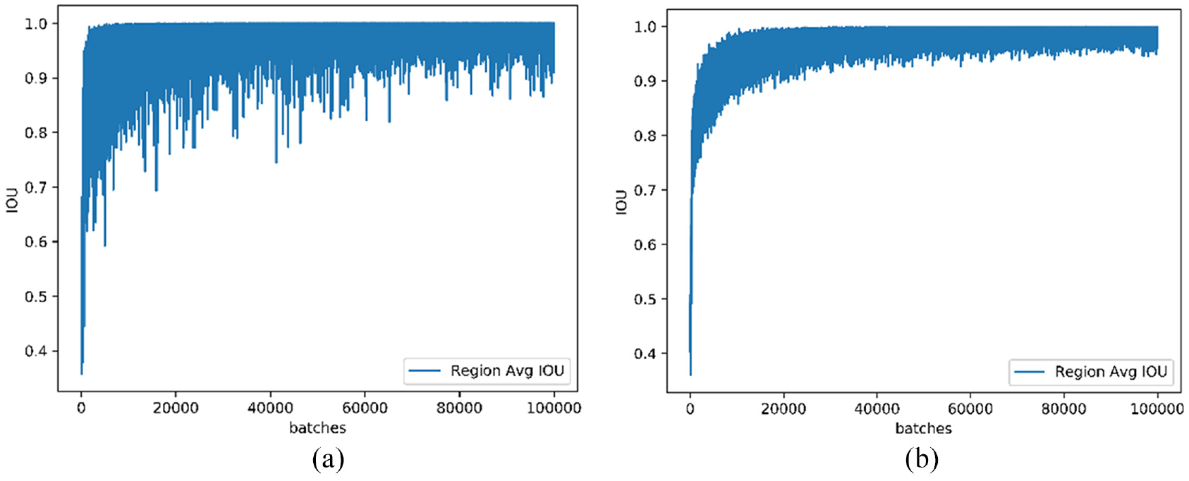
IOU accuracy curve on scales of 13×13 and 26×26: (a) scale of 13×13 and (b) scale of 26×26.

Figure 3 shows that the IOU accuracy gradually approaches the ideal value 1 from the low level of about 0.2 at the beginning for both scales. The scale of 13×13 has a small number of grids, so the error of bounding box regression will be relatively large, but the IOU accuracy will eventually stabilize at the level of about 0.9. The IOU accuracy of the scale of 26×26 is finally maintained above 0.95. Figure 4 shows some detection results using the vehicle detection network trained using YOLOv3-tiny.

Figure 4.

Some vehicle detection results on KITTI.

Experimental results show that the vehicle detection the tiny network can accurately locate the vehicle in most cases. When the road shadow blocks the vehicle or the vehicle is small in the image, there will still be missed detection. The traffic signs will be false detected as vehicles sometimes. The reason for this situation may be that the feature extractor of YOLOv3-tiny network cannot enough extract the features of the vehicle, resulting in false detection and missed detection. Furthermore, the predicted bounding box does not coincide with the true bounding box very well. In other words, the position of the vehicle is not located accurately.

Optimization of vehicle detection network

In order to improve the accuracy of the vehicle detection network, a better feature extractor is necessary. This article replaces the feature extractors in the traditional YOLOv3-tiny network by DarkNet-19 and ResNet-18 light-weight networks, respectively. They can improve the feature extraction capability of the original network without increasing the time-consuming.

DarkNet-19 network consists of 19 convolutional layers and 5 maximum pooling layers, originally proposed as a foundation feature extraction network for YOLOv2.²⁶ 1×1 convolutional kernel is utilized to compress the feature representation between 3×3 convolutional layers, which helps to speed up the convergence and normalize the model. DarkNet-19 can achieve Top 5 (91.2%) accuracy on ImageNet data set. The parameters of DarkNet-19 network are shown in Table 1.

Table 1.

Parameters of DarkNet-19.

Type	Filters	Size/stride	Output
Convolutional	32	3×3	224×224
Maxpool		2×2/2	112×112
Convolutional	64	3×3	112×112
Maxpool		2×2/2	56×56
Convolutional	128	3×3	56×56
Convolutional	64	1×1	56×56
Convolutional	128	3×3	56×56
Maxpool		2×2/2	28×28
Convolutional	256	3×3	28×28
Convolutional	128	1×1	28×28
Convolutional	256	3×3	28×28
Maxpool		2×2/2	14×14
Convolutional	512	3×3	14×14
Convolutional	256	1×1	14×14
Convolutional	512	3×3	14×14
Convolutional	256	1×1	14×14
Convolutional	512	3×3	14×14
Maxpool		2×2/2	7×7
Convolutional	1024	3×3	7×7
Convolutional	512	1×1	7×7
Convolutional	1024	3×3	7×7
Convolutional	512	1×1	7×7
Convolutional	1024	3×3	7×7
Convolutional	1000	1×1	7×7
Avgpool		Global	1000
Softmax

ResNet network was proposed by He et al.²⁷ in 2015. ResNet protects the integrity of information by directly passing the input signal to the output. It only needs to learn the difference between the input and output, simplifying the learning objective and difficulty and reducing the possibility of gradient disappearance.²⁸ Two ResNet units can be utilized to simplify the computation. Two 3×3 convolutional layers can be cascaded to form a ResNet unit. The other kind of ResNet unit is to cascade three convolutional layers in the sequence of 1×1, 3×3, and 1×1. This article adopts the ResNet-18 network as the feedforward network to optimize the performance of the vehicle detection network. ResNet network inherits the ability of the residual network to extract image features and meets the requirements of light-weighting. The structure of ResNet-18 network is shown in Figure 5.

Figure 5.

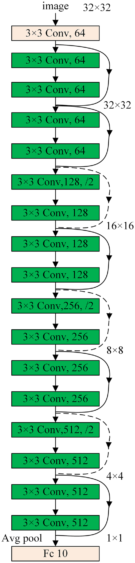
Structure ResNet-18 network.

After analyzing the false bounding boxes and missed vehicle, it is found that the width of most bounding boxes is distributed around 100 pixels and the height is around 50 pixels. Although replacing the feature extraction network of the original network can enhance the accuracy of vehicle detection, the detection performance on small vehicles is still unsatisfactory. Therefore, a scale of 52×52 is added to the original two scales (13×13 and 26×26) to improve the detection effect of the vehicle detection network for small objects. Each scale uses three anchor boxes to generate the prediction results. It is necessary to cluster nine anchor boxes on the training data using a clustering algorithm. K-means clustering algorithm²⁹ is used to generate the anchor boxes.

This article uses K-means to divide the real width and height of the bounding box into nine groups. The center of each group is taken as the parameter of the final nine anchor boxes. The detailed clustering process is as follows:

Step 1. Select clustering center points randomly as $μ_{1}, μ_{2}, μ_{3}, . . ., μ_{k} \in R^{n}$ , where k is the number of clustering centers.

Step 2. For each class i, the intersection ratio with each cluster mass is calculated, and the class of the cluster mass corresponding to the largest intersection ratio value is the class to which the sample belongs

c^{(i)} = \arg min_{j} ‖ x^{(i)} - μ_{j} ‖^{2}

(5)

where $c^{(i)}$ denotes the intersection ratio of class i, $x^{(i)}$ is the position of all samples in class i, and $μ_{j}$ is the initial clustering center of mass.

Step 3. After traversing all the samples, for each class, the median in this class is chosen to update the new initial clustering center, which can be calculated as

μ_{j} = \frac{\sum_{i = 1}^{m} 1 {c^{(i)} = j} x^{(i)}}{\sum_{i = 1}^{m} 1 {c^{(i)} = j}}

(6)

Step 4. Repeat Steps 2 and 3 until the clustering center do not change.

First, randomly select nine points as the cluster center, then calculate the intersection and union ratio of all other training data with the nine cluster centers. The cluster center with the largest intersection and union ratio is taken as the class of the training data. Then, the median of each class is calculated as the new clustering center. Continue to iterate until the cluster center does not change, and the final nine cluster centers are the final result. Figure 6 shows the final clustering result after 78 iteration times, where the red cross is the cluster center.

Figure 6.

Clustering result.

The width and height of the bounding box of each object are taken as the parameters to be clustered. The nine cluster centers in Figure 6 are [0.03163166, 0.0786631], [0.25076737, 0.47783422], [0.0430937, 0.1153877], [0.06252827, 0.16296791], [0.15647011, 0.31466578], [0.02147819, 0.05505348], [0.08710824, 0.12018717], [0.11113086, 0.19986631], and [0.05647011, 0.08312834]. The size of the input image is 416×416. The clustering result is the ratio of the width and height of the anchor box to the width and height of the original image. The parameters of the final anchor box should be transformed according to the original size, that is should be multiplied by 416. Then, the final nine cluster centers in the original input image are about [13, 33], [104, 199], [18, 48], [26, 68], [65, 131], [9, 23], [36, 50], [46, 83], and [24, 35]. The large anchor box is used to predict large objects and the small anchor box is used to predict small objects. Therefore, the three candidate boxes [46, 83], [65, 131], and [104, 1989] are used to predict bounding box on the scale of 13×13, the three candidate boxes [18, 48], [26, 68], and [36, 50] are used to predict bounding box on the scale of 26×26, and the rest three candidate boxes [9, 23], [13, 33], and [24, 35] are used to predict small bounding box on the scale of 52×52. Since the results of K-means clustering depend on the selection of initial clustering center, six clustering experiments were done in this article, as shown in Table 2.

Table 2.

Six clustering experiments with different initial clustering centers.

Number	Initial clustering center	Iteration times	Final clustering center	Size of anchor box
1	{[0.03280291, 0.10208556][0.23281906, 0.4418984 ][0.03584006, 0.10818182][0.03295638, 0.14871658][0.1827706, 0.5113369 ][0.02934572, 0.06379679][0.04668013, 0.10050802][0.07462036, 0.11435829][0.05887722, 0.07657754]}	78	{[0.03163166, 0.0786631 ][0.25076737, 0.47783422][0.0430937, 0.1153877 ][0.06252827, 0.16296791][0.15647011, 0.31466578][0.02147819, 0.05505348][0.08710824, 0.12018717][0.11113086, 0.19986631][0.05647011, 0.08312834]}	{[13, 33][104, 199][18, 48][26, 68][65, 131][9, 23][36, 50][46, 83][23, 35]}
2	{[0.29697092, 0.42139037][0.04567044, 0.07243316][0.17346527, 0.20393048][0.15427302, 0.36465241][0.02688207, 0.05491979][0.02186591, 0.07181818][0.07957997, 0.11112299][0.1369063, 0.19213904][0.27298869, 0.50229947]}	119	{[0.15728191, 0.31715241][0.04326333, 0.11604278][0.111979, 0.20093583][0.06289176, 0.16371658][0.02155089, 0.05513369][0.03180129, 0.07885027][0.05696284, 0.08360963][0.08752019, 0.12122995][0.25138934, 0.47816845]}	{[65, 132][18, 48][47, 84][26, 68][9, 23][13, 33][24, 35][36, 50][104, 199]}
3	{[0.04010501, 0.09716578][0.089063, 0.42454545][0.0915105, 0.15665775][0.15256058, 0.38850267][0.03385299, 0.11601604][0.30491922, 0.50454545][0.04630048, 0.05224599][0.03760905, 0.08697861][0.06538772, 0.07363636]}	102	{[0.04325525, 0.11601604][0.11139742, 0.20010695][0.08740711, 0.12061497][0.15686995, 0.31549465][0.06285541, 0.16358289][0.25102585, 0.4778877 ][0.02155089, 0.05513369][0.03179321, 0.07885027][0.05688207, 0.08355615]}	{[18, 48][47, 83][36, 50][65, 131][26, 68][104, 199][9, 23][13, 33][24, 35]}
4	{[0.08, 0.18588235][0.02504039, 0.05409091][0.25052504, 0.4259893 ][0.05989499, 0.12778075][0.0284168, 0.0734492 ][0.03135703, 0.09470588][0.06756058, 0.17593583][0.11528271, 0.23729947][(0.05071082, 0.20326203)]}	159	{[0.08710824, 0.12018717][0.02147819, 0.05505348][0.25076737, 0.47783422][0.05647011, 0.08312834][0.03163166, 0.0786631][0.0430937, 0.1153877][0.11113086, 0.19986631][0.15647011, 0.31466578][0.06252827, 0.16296791]}	{[36, 50][9, 23][104, 199][23, 35][13, 33][18, 48][46, 83][65, 131][26, 68]}
5	{[0.03968498, 0.04593583][0.04200323, 0.11687166][0.15747981, 0.15735294][0.04294023, 0.05331551][0.036042, 0.08409091][0.10345719, 0.22360963][0.04222132, 0.25572193][0.03246365, 0.06532086][0.05714055, 0.12676471]}	142	{[0.02147819, 0.05505348][0.06252827, 0.16296791][0.25076737, 0.47783422][0.05647011, 0.08312834][0.0430937, 0.1153877][0.15647011, 0.31466578][0.11113086, 0.19986631][0.03163166, 0.0786631 ][0.08710824, 0.12018717]}	{[9, 23][26, 68][104, 199][23, 35][18, 48][65, 131][46, 83][13, 33][36, 50]}
6	{[0.09589661, 0.16395722][0.03155897, 0.08617647][0.07442649, 0.19628342][0.1753958, 0.23459893][0.05424071, 0.12836898][0.08084006, 0.165][0.02853796, 0.07572193][0.02140549, 0.05382353][0.21005654, 0.47128342]}	48	{[0.10693053, 0.18501337][0.03977383, 0.08465241][0.06471729, 0.16652406][0.15327544, 0.3][0.04610662, 0.12264706][0.07534733, 0.10513369][0.02747173, 0.07128342][0.01965267, 0.05024064][0.24643376, 0.47635027]}	{[44, 77][17, 35][27, 69][64, 125][19, 51][31, 44][11, 30][8, 21][103, 198]}

The vehicle detection network optimized using feedforward network and multi-scale clustering is as shown in Figure 7. The backbone network sends the extracted 13×13 features to the neck network, and the up-sampling multiplier of ×1, ×2, and ×4 to get 13×13, 26×26, and 52×52 size features, respectively, and then sends these different size features to different head networks to detect targets at different scales.

Figure 7.

Structure of optimized vehicle detection network.

Experiments and results

To evaluate the performance of the optimized vehicle detection network, the accuracy P and the recall R are defined to evaluate the performance of the network. They can be calculated as

{\begin{matrix} P = \frac{TP}{TP + FP} \\ R = \frac{TP}{TP + FN} \end{matrix}

(7)

where TP, FP, and FN denote the number of true positives, number of false positives, and number of false negatives, respectively. TP means that the vehicle on the road can be recognized and the classification is consistent with the actual type. FP means that the vehicle is recognized but the classification is not consistent with the actual type, or the background such as billboard is recognized as the vehicle. FN means that there is a vehicle in the image, but it is not recognized accurately.

Define the average accuracy as mAP, which denotes the area enclosed by the P–R curve and the coordinate axis. It can be calculated as

mAP = \int_{0}^{1} P (R) d R

(8)

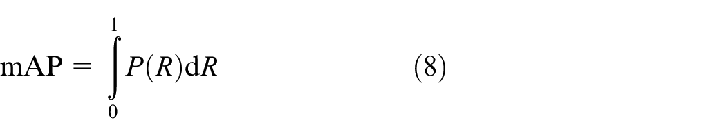
The ideal value of mAP is 1. The closer of mAP value is to 1, the higher the detection accuracy of the model. The P–R curves of the traditional and optimized vehicle detection network are shown in Figure 8.

Figure 8.

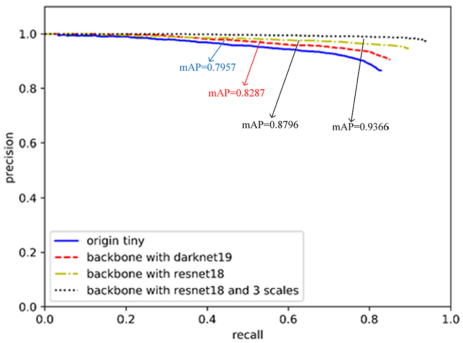
P–R graph for each network.

Figure 8 shows that the mAP of the traditional YOLOv3-tiny network is 79.57%. After using the DarkNet-19 as the feedforward network to replace the feature extractors of the traditional YOLOv3-tiny network, the mAP is 82.87%. While using the ResNet-18 to replace the feature extractors of the traditional YOLOv3-tiny network, the mAP is 87.96%, which is better than the DarkNet-19. The proposed vehicle detection network optimized by adds multi-scale prediction to ResNet-18 as the feedforward network, the mAP is 93.66%, which has an improvement of 14.09% compared with the traditional YOLOv3-tiny network.

Some of the results are shown in Figure 9. The green box in the figure shows the results of the traditional YOLOv3-tiny network, and the red box shows the results of the proposed vehicle detection network.

Figure 9.

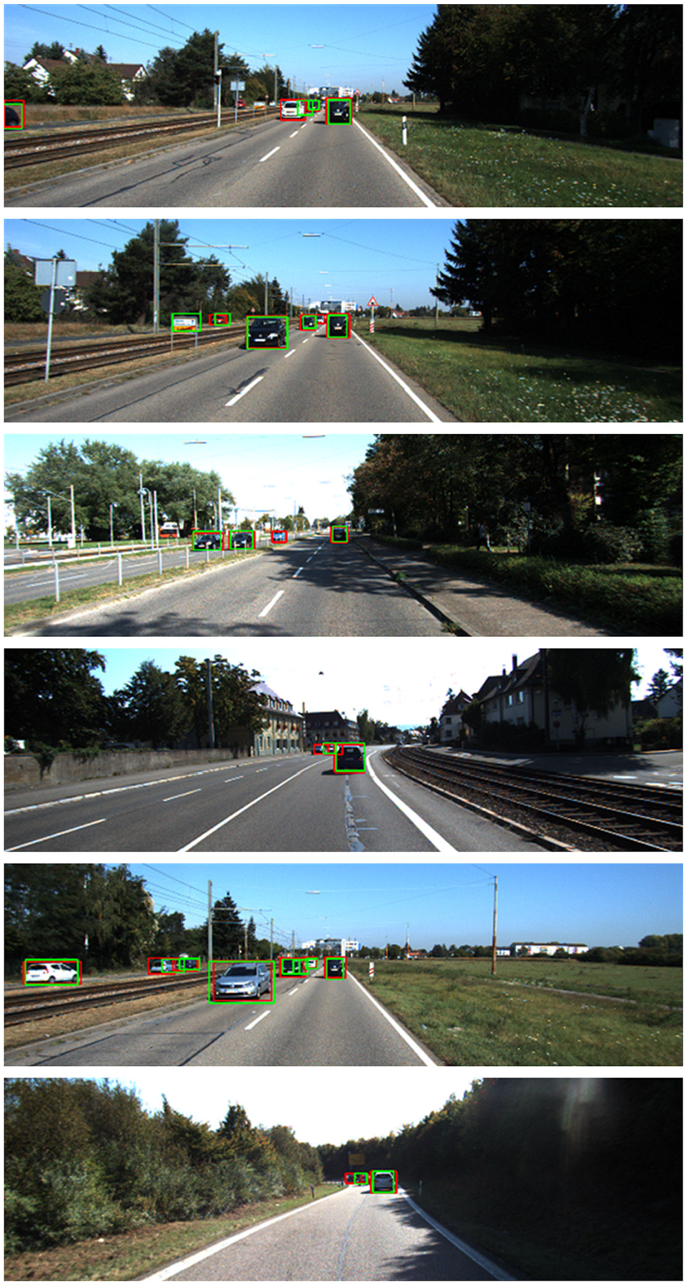
Comparison of some detection results after optimized.

Figure 9 indicates that our improved method can show a high robustness to detect small object. The improved algorithm can detect small vehicles that cannot be detected by the original algorithm, and the bounding boxes generated by the improved algorithm are more accurate.

To evaluate the performance of the proposed vehicle detection network, several tests were conducted on the embedded platform TX2 and laptop. TX2 is an embedded artificial intelligence computing platform launched by NVIDIA in 2018 with Pascal architecture. GPU and CPU are consisted of two Denver and four A57 cores together. The laptop has a graphics card of NVIDIA GTX1060 6G and an Intel i7-7700HQ processor. The comparison result of each network is shown in Table 3.

Table 3.

Comparison of different networks on embedded device.

Network model	TX2 (fps)	Laptop (fps)	mAP (%)	Model size (MB)
YOLOv3-tiny	24	63	79.57	34.7
YOLOv3-tiny with DarkNet-19	10	45	82.87	91.2
YOLOv3-tiny with ResNet-18	15	60	87.96	53.0
Optimized network with ResNet-18 and multi-scale	13	60	93.66	55.6

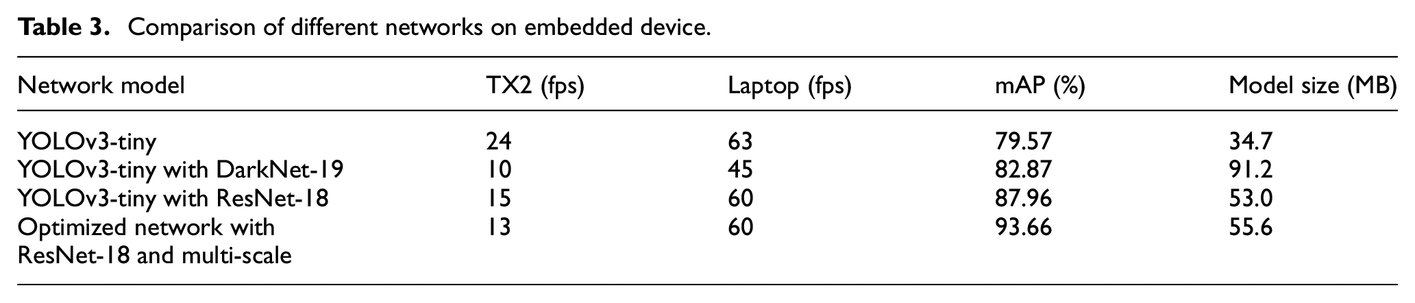
Table 3 indicates that the traditional YOLOv3-tiny network has the simplest structure and the least number of parameters, and it can run at 24 fps on an embedded device. However, the detection accuracy is only 79.57%. While using the ResNet-18 to replace the feature extractors of the traditional YOLOv3-tiny network, it can run at speed on embedded devices with an accuracy of 87.96%, which is 8.39% higher than the traditional YOLOv3-tiny network. It can still reach 60 fps on the laptop. After adding multi-scale prediction to ResNet-18, the network runs at a similar speed and the size only increases by 2.6 MB. However, the detection accuracy improves by 5.7%. It can be seen that after two different levels of optimization, although the structure and the number of parameters becomes larger, and the speed of operation in the embedded hardware decreases. The detection accuracy improves from 79.57% to 93.66%, and it can reach 13 fps on embedded devices.

Conclusion

Vehicle detection methods based on deep learning show superiority over the traditional feature-based and machine learning-based methods. This article utilizes the traditional YOLOv3-tiny as the base network, proposed a light-weighted vehicle detection using the KITTI data set. Facing the poor vehicle detection accuracy of YOLOv3-tiny network, two light-weight models, DarkNet-19 and ResNet-18, were used to replace the original feature extraction network of YOLOv3-tiny. The detection accuracy increased from 79.57% to 87.96% when taking ResNet-18 to realize feature extraction. However, the detection of small objects is still poor, and the strategy of multi-scale is proposed. The K-means algorithm is utilized to cluster nine anchor boxes in three scales; they are 13×13, 26×26, and 52×52. Experimental results show that multi-scale strategy can effectively improve vehicle detection accuracy. The optimized vehicle detection light-weight network was tested on the embedded device TX2 and laptop. It was verified that the optimized network not only has improved detection accuracy, but also can meet the requirement of real-time.

In the follow-up work, we will further study the optimization of network and reduce time consumption. At the same time, more experiments and comparisons are helpful to reflect the superiority of our work. It is a huge challenge for application in real traffic environment; more data sets need to be supplemented to deal with the changeable objects under different situations.

Footnotes

Handling Editor: Peio Lopez Iturri

Declaration of conflicting interests

The author(s) declared no potential conflicts of interest with respect to the research, authorship, and/or publication of this article.

Funding

The author(s) disclosed receipt of the following financial support for the research, authorship, and/or publication of this article: This work is partially supported by the National Natural Science Foundation of China (grant nos 51975089 and 52175078) and the Natural Science Foundation Program of Liaoning Province (grant no. 2021-MS-127).

ORCID iD

Lie Guo

References

National Bureau of Statistics of the People’s Republic of China. Annual statistics of the National Bureau of statistics of the People’s Republic of China in 2020, http://data.stats.gov.cn/

Nguyen

Kajita

Traffic congestion and impact on the environment in Vietnam: development of public transport system—experience from actual operation of bus in Hanoi. J Civil Environ Eng 2018; 8: 317.

Zhu

Yuen

Mihaylova

, et al. Overview of environment perception for intelligent vehicles. IEEE T Intell Transp 2017; 18: 2584–2601.

Wang

Cai

, et al. Soft-weighted-average ensemble vehicle detection method based on single-stage and two-stage deep learning models. IEEE Trans Int Veh 2021; 6: 100–109.

Lee

Lim

Kwon

, et al. Stereo vision-based vehicle detection using a road feature and disparity histogram. Opt Eng 2011; 50: 027004.

Aqel

Hmimid

Sabri

, et al. Road traffic: vehicle detection and classification. In: 2017 intelligent systems and computer vision (ISCV), Fez, Morocco, 17–19 April 2017, pp.1–5. New York: IEEE.

Noh

Shim

Jeon

Adaptive sliding-window strategy for vehicle detection in highway environments. IEEE T Intell Transp 2016; 17: 323–335.

Nguyen

Multiscale feature learning based on enhanced feature pyramid for vehicle detection. Complexity 2021; 2021: 5555121.

Zhang

Zheng

Gao

, et al. Part-aware region proposal for vehicle detection in high occlusion environment. IEEE Access 2019; 7: 100383–100393.

10.

Garg

Nie

, et al. A highly efficient vehicle taillight detection approach based on deep learning. IEEE T Intell Transp 2021; 22(7): 4716–4726.

11.

Chen

Lin

. Embedded system real-time vehicle detection based on improved YOLO network. In: 2019 IEEE 3rd advanced information management, communicates, electronic and automation control conference (IMCEC), Chongqing, China, 11–13 October 2019, pp.1400–1403. New York: IEEE.

12.

Girshick

Donahue

Darrell

, et al. Rich feature hierarchies for accurate object detection and semantic segmentation. In: 2014 IEEE conference on computer vision and pattern recognition, Columbus, OH, 23–28 June 2014, pp.580–587. New York: IEEE.

13.

Redmon

Divvala

Girshick

, et al. You only look once: unified, real-time object detection. In: 2016 IEEE conference on computer vision and pattern recognition (CVPR), Las Vegas, NV, 27–30 June 2016, pp.779–788. New York: IEEE.

14.

Liu

Anguelov

Erhan

, et al. SSD: single shot multibox detector. In: Leibe

Matas

Sebe

, et al. (eds) Computer vision—ECCV 2016. Cham: Springer International Publishing, 2016, pp.21–37.

15.

Ren

Girshick

, et al. Faster R-CNN: towards real-time object detection with region proposal networks. IEEE Trans Pattern Anal 2017; 39: 1137–1149.

16.

Guo

Wang

, et al. An accurate and fast single shot multibox detector. IET Comput Vis 2020; 14: 391–398.

17.

Tajar

Ramazani

Mansoorizadeh

A lightweight tiny-YOLOv3 vehicle detection approach. J Real-Time Image Pr 2021; 18(6): 2389–2401.

18.

Feng

, et al. Fast and accurate detection of kiwifruit in orchard using improved YOLOv3-tiny model. Precis Agric 2021; 22(3): 754–776.

19.

Haq

Muhammad

Hussain

, et al. Movie scene segmentation using object detection and set theory. Int J Distrib Sens N 2019; 15: 1550147719845277.

20.

Elgendy

Sik-Lanyi

Kelemen

A novel marker detection system for people with visual impairment using the improved tiny-YOLOv3 model. Comput Meth Prog Bi 2021; 205: 106112.

21.

Redmon

Farhadi

YOLOv3: an incremental improvement. arXiv preprint arXiv 2018: 1804.02767, https://arxiv.org/pdf/1804.02767.pdf

22.

Song

Pan

Gao

, et al. Improved non-maximum suppression for object detection using harmony search algorithm. Appl Soft Comput 2019; 81: 105478.

23.

Cheng

Zheng

, et al. Multi-scale safety helmet detection based on SAS-YOLOv3-tiny. Appl Sci 2021; 11(8): 3652.

24.

Geiger

Lenz

Urtasun

. Are we ready for autonomous driving? The KITTI vision benchmark suite. In: 2012 IEEE conference on computer vision and pattern recognition, Providence, RI, 16–21 June 2012, pp.3354–3361. New York: IEEE.

25.

Song

Liang

, et al. Vision-based vehicle detection and counting system using deep learning in highway scenes. Eur Transp Res Rev 2019; 11: 51.

26.

Sang

Zhang

, et al. Multi-scale vehicle detection for foreground-background class imbalance with improved YOLOv2. Sensors 2019; 19: 3336.

27.

Zhang

Ren

, et al. Deep residual learning for image recognition. In: 2016 IEEE conference on computer vision and pattern recognition (CVPR), Las Vegas, NV, 27–30 June 2016, pp.770–778. New York: IEEE.

28.

Cao

Shen

Estimating depth from monocular images as classification using deep fully convolutional residual networks. IEEE T Circ Syst Vid 2018; 28: 3174–3182.

29.

Baruri

Ghosh

Banerjee

, et al. An empirical evaluation of k-means clustering technique and comparison. In: 2019 international conference on machine learning, big data, cloud and parallel computing (COMITCon), Faridabad, India, 14–16 February 2019, pp.470–475. New York: IEEE.

Light-weighted vehicle detection network based on improved YOLOv3-tiny

Abstract

Keywords

Introduction

Vehicle detection light-weighted network

Vehicle detection network YOLOv3-tiny

Optimization of vehicle detection network

Experiments and results

Conclusion

Footnotes

Declaration of conflicting interests

Funding

ORCID iD

References